
Soft Actor Critic: Deep Reinforcement Learning for Robotics?
Motivation and introduction
The Soft Actor-Critic algorithm by Haarnoja et al. [1] has gotten a lot of coverage and attention in 2018 and 2019. And rightfully so. The paper proposes a very elegant solution to the notorious problem of deep reinforcement learning algorithms being too data-hungry for real-world feasibility and supplies very exciting examples illustrating the capabilities of the algorithm in a real-world setting, as can be seen below. Naturally, I was intrigued. While at the point of writing this post, Reinforcement Learning has not yet been featured on this site, it is, after all, my main academic interest and will be at the heart of my masters’ (and hopefully Ph.D.) thesis. Hence, for one of my courses, I decided to write a paper on the Soft Actor-Critic algorithm. In this blog post, I built on that paper [2] and provide some additional examples and insights.
The problem with Deep Reinforcement Learning for real world robotics
While this post will not address Reinforcement Learning in general, the gist of it is as follows: By executing pseudo-random actions in an environment (or simulation thereof) and rewarding good actions, we can have a, for example robotic, agent learn almost any desired behavior. Here, behavior means that we execute the desired sequence of actions to get from some initial state to some goal state. Inherently, this is a very powerful concept, as this makes it possible for robots to learn how to walk, grasp things, play games, engage in dialogue, and pretty much learn to solve any conditional, sequential problem. That’s the theory, at least.
However, as you might have noticed, we are not yet surrounded by intelligent, autonomous robots in our everyday life, in fact, it’s still out of the norm to find a robot autonomously cleaning an office space or shopping mall, which indicates that things aren’t quite as easy. Many different fields of robotics are still active research areas, just like Reinforcement Learning is still having a central problem, stopping it from being widely employed in real-world robotic scenarios. To be precise, the main problem of deep Reinforcement Learning algorithms for real-world robotics is that they are insanely data-hungry and take ages to converge (ie manage to generate the desired behavior).
Why is this problematic? Well, robots aren’t indestructible and in the early stages of learning, Reinforcement Learning agents behave essentially randomly. You can probably imagine what drastic consequences it can have if we just set all motors in our robot to random power levels… Larger robots will fall over, mobile bots might severely ram into obstacles, and drones would crash immediately. If we expose our robots to this kind of behavior for a prolonged period of time, it is almost certain that the robot will suffer significant damage in the process (similar to how toddlers fall over when they begin learning to walk, except here, consequences aren’t inevitable breakdown). And this is only one aspect of the issue. When I wrote insanely data-hungry, I absolutely meant that. For example, AlphaStar, DeepMind’s deep neural Reinforcement Learning algorithm, has been with trained many agents in parallel, for 14 days straight, on 16 Tensor Processing Units (TPU), corresponding to 200 years of real-life training time, for each agent [3]… And this is under the employment of state-of-the-art methods to speed up the learning process.
Ignoring that we can’t train a single robot in parallel fashion, after 200 years of hypothetical training, you can be sure that the robot would have broken down simply due to all the wear and tear that it would be exposed to in all that time.
An apparent solution is to train the agent in a simulator (which also allows us to parallelize the training process) and then simply put the behavior policy learned in the simulation on a physical robot, operating in the real world. However, the simulators are not yet good enough and fail to accurately represent the real world, which makes the learned behavior policies useless on the real, physical robot. Further, agents trained in a simulator tend to learn things that are hyper-specific to that simulator and don’t generalize to the real world. This is referred to as the Sim-to-Real problem and is an active research area in itself.
So as you can see, there are a lot of challenges for real-world Reinforcement Learning. However, the Soft Actor-Critic algorithm tackles the problem at its root and aims to significantly speed up the learning process, to a point where deep Reinforcement Learning methods become feasible in real-world scenarios. Let’s explore the intuition behind the algorithm in the following section.
The intuition behind Soft Actor Critic
To gain an understanding into how the SAC algorithm tackles the data inefficiency problem of deep Reinforcement Learning methods, we have to look at the SAC specific reward function that is being employed by Haarnoja et al. However, to begin with, consider the classical Reinforcement Learning object, that describes the general goal of Reinforcement Learning [9]: $$G_t = \sum^\infty_{k=0}\gamma^k R_{t+k+1}$$ This is the expected discounted return \(G\) at time step \(t\), with a discount factor \(0 \le \gamma \le 1\), so that the reward signal \(R\) from \(t+k+1\) time steps in the future is weighted to be less important than the reward signal at \(t+k\), encoding an aspect of temporal relevance. The reward signal \(R\) is, arguably, the central part of any Reinforcement Learning problem, as this guides what the policy (always denoted by \(\pi\)) of our agent will learn, by encoding the goodness of any action taken. Generally, the behavior, which is encoded in the policy of the agent, is adapted in such a way that it maximizes the reward function, thus, a well thought out reward function is the key for success in reinforcement learning. Essentially, no matter what, with Reinforcement Learning, we want to accumulate as much discounted reward, aka return \(G_t\) as possible. This is the main objective all Reinforcement Learning methods are subject to. Formally, the optimal policy \(\pi^*\) is defined as the policy that has the highest expected reward for every action, at every timestep, in every state [1]: $$\pi^* = \underset{\pi}{\operatorname{argmax}} \underset{\tau \sim \pi}{\mathbb{E}} \left[ \sum^\infty_{t=0} \gamma ^t [r(s_t, a_t)]\right]$$ Here, (\( \tau \sim \pi\)) means that a trajectory of interactions (\(\tau \)) has been sampled (\(\sim \)) from the probability distribution of the policy (\(\pi\)). Notice that \(r\) is a function, over all states and actions, providing the reward meassure of goodness for every combination of states and actions (at least in simple examples).
Now, the central element in the SAC algorithm is an advanced, general reward function, that contains a second term in addition to the main reward signal [7]: $$\pi^* = \underset{\pi}{\operatorname{argmax}} \underset{\tau \sim \pi}{\mathbb{E}} \left[ \sum^\infty_{t=0} \gamma ^ t [r(s_t, a_t) + \alpha \mathcal{H}(\pi(\cdot | s_t)] \right]$$ The only difference to the original formula for the optimal policy is the term \(\mathcal{H}\), which is weighted by \(\alpha\). \(\mathcal{H}\) encodes the entropy of the policy \(\pi\) in every state and is given by \(\mathcal{H}(P) = \underset{x \sim P}{\operatorname{\mathbb{E}}} [-log P (x)]\). Entropy is, roughly speaking, a meassure of information gain or uncertaintaniy of a random variable \(x\), sampled from a distribution \(P\). Do you see what this motivates the Reinforcement learning agent, who behaves according to a learnt policy that maximizes the given function, to do? It forces the agent to not only consider the reward associated with an action in a state, but also the overall degree of uncertainty in that state. This results in the agent choosing actions that lead to states which have not yet been seen, especially when a different action would lead to a state that has a higher expected return (but has already been seen). The parameter \(\alpha > 0\) balances the two components of the objective function and controls the importance of the entropy term, compared to the reward signal. In the original version of the SAC algorithm, this parameter \(\alpha\) had to be set manually, which was a non-trivial problem for complex enough environments and required an expensive hyperparameter optimization [1]. However, in the newer version of the algorithm, Haarnoja et al. managed to automatically adjust the parameter by rephrasing the objective function once again. However, the details of this automatic temperature adjustment can be ignored for the purpose of this blog post.
In addition to speeding up the overall learning process and making for better data efficiency, this RL objective function has another desirable side effect: It produces much more stable policies [1], [7]. Unfortunately, it is not further explained why that is, but I think about it like this: Since the reward for every state also depends on the entropy component, the agent is less likely to visit the same state twice because the entropy for that state will already be decreased. Hence, by exploring many, slightly different trajectories (sequences of states and selected actions), the overall policy is more robust, because it does not hinge on observing a small amount of key states in order to be able to select the overall best action. I hope that makes sense...? But those are just my two cents... Either way, in the video above, we can observe the consequences of this: The agent can deal with significant perturbations of the state (brick wall, stairs, ramp) that it has not encountered during training. This is a very nice property to have, as it implies that the learned policy is more general and can be employed in contexts that are not part of the training data.
And this is how far I will go regarding the basic idea behind the SAC algorithm. To summarize, SAC incorporates an entropy term into the Reinforcement Learning objective function, which motivates the agent to select actions under consideration of the uncertainty associated with each state. Like this, the agent can explore the environment much more efficiently, which results in significantly faster convergence, compared to many other state-of-the-art algorithms (see the original paper for benchmarking results [1]). For the remainder of this post, we will explore and discuss how the algorithm performs on a practical OpenAI Gym task.
OpenAI Gym example

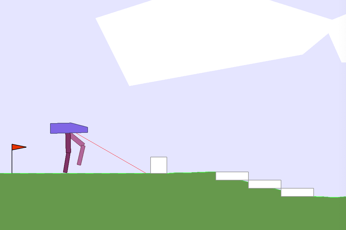
OpenAI Gym [4] provides a wide array of Reinforcement learning environments and is one of the de-facto tools being used to benchmark, compare and develop Reinforcement Learning algorithms. For getting practical experience with the SAC algorithm, I selected the BipedalWalker environment, where the goal is for a bipedal agent to develop an efficient walking gait. This environment is particularly interesting, for reasons further explained below, because it has a normal and a hardcore version, where the hardcore version of the environment contains many stumps, pitfalls, and stairs and is much harder to solve successfully. As we can see in the above video, the walking gait learned on the minotaur robot appears to be outstandingly stable, generalizing to a handful of unseen scenarios: The brick wall and the ramp. So my hypothesis is as follows: The bipedal walker trained on the normal version of the environment might be robust enough to also solve the hardcore version of the environment, similar to how the minotaur in the video could deal with the obstacles presented in the testing scenarios! To investigate this hypothesis, we need a working version of the algorithm though. Instead of implementing this algorithm from scratch (which would take a lot of time and straight-up not be efficient), we will use the implementation provided in this repository [5].
Results
To begin with, I trained a SAC agent for 500 epochs on both the normal and hardcore version of the environment. For comparison, I also trained a PPO [6] agent and a TD3 [8] on both versions of the environment, to put the convergence time of the SAC agent into perspective. To be fair, PPO is an on policy method, which are known to have much worse data efficiency than off-policy methods. Consider the results presented below:
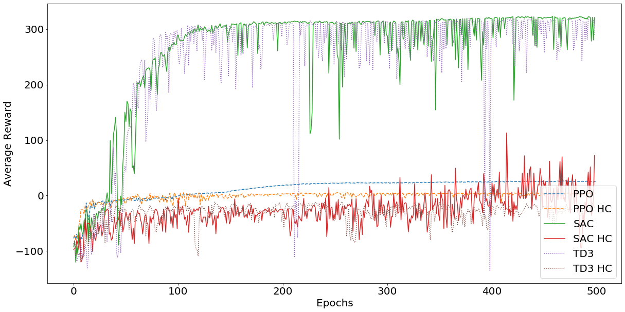
We can observe that on the normal version of the environment, the algorithm converges within roughly ~ 100 epochs of 5000 interactions with the environment per epoch. However, out of the box, the algorithm does not appear to be able to solve the hardcore version of the environment within 500 epochs. Based on this data alone, I can not really draw further conclusions. It is very well possible that with slight adjustments to the hyperparameters, a SAC algorithm could solve the hardcore version of the environment as well. However, not wanting to invest more time into this blog post, I did not bother to conduct an expensive and timely hyperparameter optimization and applied the algorithm with its out-of-the-box configuration to both versions of the environment. Further, we can observe that the TD3 agent learns just as fast as the SAC agent. Again, we can’t really conclude anything beyond that this is how these algorithms perform, given this exact scenario and hyperparameter configuration. The benchmarking results presented by Haarnoja et al. do more justice to the efficiency of the algorithm than this small experiment and I highly encourage taking a look at the paper [1].
Interestingly enough, TD3 struggles to make meaningful progress within 500 episodes on the hardcore version of the environment as well. This gives some indication of the difficulty associated with this specific environment. As expected, the PPO agent hasn’t come close yet to solving the environement, which it would likely do, given more training data
To begin the analysis of our main hypothesis, whether the policy learned by the SAC agent is robust enough to be transferred from the normal version of the environment to the hardcore one, consider the below Figure:
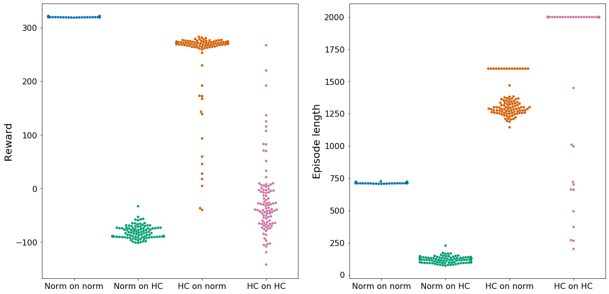
These statistics tell us a few things on how the learned policies perform, already regarding the main hypothesis we sought out to investigate, whether policies trained on the simple version of the environment would be robust enough to also deal with the obstacles presented in the hardcore version of the environment, without encountering them during training. Sadly, a short glance at Figure 3 immediately falsifies that hypothesis. We can observe that when executing the policy trained on the normal version of the environment on the hardcore version, we get an average reward of roughly -100, with low deviations from that value. This is because the environment punishes the agent with a -100 reward when it falls over. Hence, the policy learned on the normal version of the environment is not robust enough to get past the obstacles in the hardcore version and falls over, getting punished with a -100 reward. Further, we can observe that the agent trained on the normal version of the environment does not appear to have a deviation from the reward and episode length. This indicates that the agent performs equally well (or badly) most of the time, contrary to the agent trained on the hardcore version of the environment. There, we can observe a much higher range of values, indicating external factors (aka the obstacles) having an effect on the performance of the agent. To further verify our conclusion regarding our main hypothesis, take a look at how the agent performs in practice:
As expected, the agent developed a (kinda awkward looking) walking gait, that successfully solves the normal version of the environment by traveling all the way to the end of the level. This is the most efficient gait it found, as applying torque to the joints costs a small amount of reward. Regarding our main hypothesis, consider the following video, where we employ the policy trained on the normal version of the environment on the hardcore version:
Here, we can see how the agent struggles to get past the obstacles. This properly rejects (I think conducting a T-Test on the reward distribution would be overkill and is not necessary for this blog post) our hypothesis: A SAC agent trained on the normal BipedalWalker environment is not robust enough to also solve the BipedalWalkerHardcore environment, as already indicated in Figure 3. In hindsight, I see how this is too big of a leap from the normal to the hardcore version of the environment. There is a clear difference to the real-world examples we saw above: In the examples with the stairs, the ramp, and the small brick wall, the robot, controlled by the learned policy, gets away with just sticking to the learned policy. These obstacles don’t require dedicated handling, the robot does not have to learn a specific behavior to get past them. The obstacles faced in the hardcore version of BipedalWalker environment can clearly not be handled in the same way. The agent needs to find a distinct strategy for dealing with the different obstacles present in the hardcover version of the BipedalWalker environment.
So what about the SAC agent that has been trained directly on the hardcore version of the environment? Well, take a look…
As you can see, that agent performs very poorly. However, I am certain that the agent would learn how to get past the different hurdles given a) more training time/data and or b) a hyperparameter optimization for that version of the environment. We can see already that the walking gait, if we can call it that, differs from what was learned on the normal version of the environment. This becomes even more apparent when we visualize the two agents side by side, one having been trained on the normal version of the environment, the other on the hardcore version:
Extra
Purely because it’s somewhat interesting too look at, here is a video of the walking gaits developed by the TD3, PPP and SAC algorithm (SAC trained on normal and HC environment):
Summary
Alright, wrapping it up: Deep Reinforcement Learning methods suffer from strong data inefficiency. The Soft Actor-Critic algorithm by Haarnoja et al. tackles this data inefficiency problem of (deep) Reinforcement Learning algorithms, by modifying the reward object to include an entropy regularization term. Haarnoja et al. provide real-world examples demonstrating strong robustness of the developed policies and strong benchmarking results. We sought ought to investigate whether a SAC policy learned on the normal version of the environment would be robust enough to clear the obstacles in the hardcore version of the environment. Our results clearly indicate that this is not the case, for reasons provided above.
Finally, I want to mention that Haarnoja et al. are of course not the only people investigating data inefficiency in deep reinforcement learning methods. Here are a few approaches, in case you want to do some additional googling: Task Simplification, Imitation Learning, Hindsight imagination, Hierarchical Reinforcement Learning…
All data and code is available here.
Cheers,
Finn.
References:
[1] Soft Actor Critic Algorithms and Applications, Haarnoja et al.
[2] My coursework paper on the SAC algorithm
[3] DeepMind’s AlphaStar
[4] OpenAI Gym
[5] Createamind DRL: SAC implementation
[6] Proximal Policy Optimization Algorithms
Soft Actor-Critic: Off-Policy Maximum Entropy Deep Reinforcement Learning with a Stochastic Actor
[8] Addressing Function Approximation Error in Actor-Critic Methods
[9] Sutton and Barto: Reinforcement Learning: An Introduction