
Multi-Objective Deep Reinforcement Learning with Lexicographic Task-priority constraints
Motivation and introduction
Deep Reinforcement Learning (RL) Doesn’t Work Yet. That’s what Alexander Irpan wrote in his famous blog post back in 2018. Sadly, 5 years later, RL researcher and practitioners are still struggling with the same challenges that Alexander Irpan wrote about 5 years ago. Although we had some exciting advances and innovations, e.g. the Dreamer algorithm series, Decision Transformer, and SayCan, I believe most practitioners would agree with the following statements, which, in one way or another, have also been made by Alexander Irpan:
- DRL algorithms, that learn to solve each task from scratch, are still very sample inefficient, often requiring millions of transitions before achieving acceptable levels of performance.
- Designing scalar-valued reward functions for complex tasks that induce the desired behavior is difficult, with few general heuristics available.
- The inherent unsafe exploration of trial-and-error-based learning algorithms and the blackbox-natures of the resulting DNN-based agents hinders the more widespread employment of DRL in real-world applications.
Fortunately, with our recent paper (“Prioritized Soft Q-Decomposition for Lexicographic Reinforcement Learning”), we address all of these pain points, at least to some extent.
So, this hopefully got you interested in our work.
In the next sections, I will provide an informal summary of our paper, starting with a recap of Multi-Objective Reinforcement Learning (MORL).
Multi-Objective Reinforcement Learning
In our paper, we want to solve special MORL problems, but we begin with a general definition of MORL problems. MORL problems are formalized by a Markov decision process (MDP), \(\mathcal{M} \equiv (\mathcal{S, A}, \mathbf{r}, p, \gamma)\), where \(\mathcal{S \in \mathbb{R}^k, A \in \mathbb{R}^l}\) respectively denote the state- and action-space, \(\mathbf{r}: \mathcal{S} \times \mathcal{A} \to \mathbb{R}^n\) denotes a vector-valued reward function, \(p\) denotes the transition dynamics, and the discount factor is given by \(\gamma \in [0, 1]\). Importantly, in MORL, each dimension \(i\) of the vector-valued reward function \(\mathbf{r}(\mathbf{s},\mathbf{a})\) corresponds to a scalar-valued subtask reward function, meaning we have \(\mathbf{r}(\mathbf{s},\mathbf{a})_{[i]} = r_i(\mathbf{s},\mathbf{a}) \in \mathbb{R}\). Further, directly maximizing the vector-valued reward function is usually not possible, since we can’t determine a unique, optimal policy for a vector-valued reward function. For this reason, MORL algorithms usually rely on scalarization: The vector-valued reward function can be scalarized via some weighted sum (not all problems can be modeled this way), then the resulting scalar-valued reward function \({r}(\mathbf{s}, \mathbf{a}) = \sum_{i=1}^n \beta_i r_i(\mathbf{s}, \mathbf{a})\) can be maximized with any classical RL algorithm. Building on this formalism, in the next section we introduce lexicographic MORL problems, which are the particular kinds of MORL problems we are interested in.
Lexicographic MORL
In our paper, we are interested in solving special MORL problems, with continuous state- and action-spaces, like multi-objective robot control problems. In particular, the special MORL problems we are interested in are referred to as lexicographic or task-prioritized MORL problems. These are MORL problems where the subtasks are ordered by priority, meaning lexicographic MORL problems can model that some subtask \(r_i\) is more important or of higher priority that some other subtask \(r_j\). In this blog post and in our paper, we use the symbol \(\succ\) (“succeeds”) to denote anything involving lexicographic task priorities. For example, \(r_{1\succ2}\) means a lexicographic MORL task where subtask \(r_1\) is of higher priority than subtask \(r_2\). Formally, a lexicographic MORL problem is given an MDP \(\mathcal{M}_\succ \equiv (\mathcal{S, A}, \mathbf{r}, p, \gamma, o, \varepsilon)\), where \(o = \langle 1, 2, \dots i \dots n \rangle\) specifies the priority-order of subtasks and \(\varepsilon = \langle \varepsilon_1, \varepsilon_2, \dots \varepsilon_i \dots \varepsilon_n \rangle\) are certain threshold variables (more on those later). Thus, lexicographic MORL makes for a natural and intuitive way of specifying task complex tasks, by specifying a priority order of simpler subtasks. Arguably, this is more convenient and more intuitive than carefully designing a scalar-valued reward function that induces some complex behavior.
Solving a lexicographic MORL problem means finding a policy that is optimal for the highest-priority subtask, while for each lower-priority subtask, it is as good as possible while subject to the constraint of not worsening the performance of any of the higher-priority subtasks. More formally, this means that policy search for each subtask \(i\) is constrained to a set \(\Pi_i\), which contains only those policies that are also optimal for each higher priority task \({1, \dots, i-1}\).
In practice, we allow for some worsening of higher-priority subtask performance \(J\), since otherwise, the set \(\Pi_i\) would only contain the optimal policies for the higher-priority subtasks. How much we allow the performance of higher-priority subtasks to worsen is defined by the aforementioned \(\varepsilon_i\) thresholds. Thus, in a lexicographic MORL problem, policy search for subtask \(i\) is constrained to the set
\[\Pi_{i} = \{ \pi \in \Pi_{i-1} \mid \underset{\pi' \in \Pi_{i-1}}{\max} J_{i-1}(\pi') - J_{i-1}(\pi) \le \varepsilon_{i-1} \}. \tag{1}\]Unfortunately, computing the set \(\Pi_i\) and performing policy search is intractable for continuous state-action-space MDPs. However, there are other ways for optimizing policies subject to lexicographic task-priority constraints, as we will see in Section Our method: Prioritized Soft Q-Decomposition. Before we can describe our algorithm, however, we require the following two, additional background sections.
Q-Decomposition
A useful technique for solving (lexicographic) MORL problems is Russell and Zimdar’s Q-Decomposition formulation. The paper states that for scalarizable, vector-valued reward functions, the Q-function can be decomposed into \(n\) local Q-functions, each corresponding to one subtask. This means that for the \(n\) subtask reward functions in \({r}(\mathbf{s}, \mathbf{a})\) and a policy \(\pi\), we can learn \(n\) Q-functions
\[Q_i^\pi (\mathbf{s}, \mathbf{a}) = r_i(\mathbf{s}, \mathbf{a}) + \gamma Q_i(\mathbf{s}', \pi(\mathbf{s}')), \forall i \in \{1,\dots,n\} \tag{2}\]and reconstruct the Q-function for the overall, scalarized MORL problem as
\[{Q}^\pi = \sum_{i=1}^n \beta_i Q_i^\pi(\mathbf{s}, \mathbf{a}). \tag{3}\]This result is useful because it allows us to learn these Q-functions separately and concurrently (with some caveats like the tragedy of the commons, more on this later). Furthermore, we can potentially transfer and re-use the constituent Q-functions \(Q_i^\pi(\mathbf{s}, \mathbf{a})\) for different MORL tasks. Lastly, the decomposed nature of the Q-Decomposition methods benefits the interpretability of the RL agent, since we can inspect the different components that jointly induce the behavior of the agent, which is not the case with classical, non-decomposed agents. Due to these desirable attributes of the Q-Decomposition method, we are building on and extending the Q-Decomposition framework in our paper. In particular, we extend Q-Decomposition to soft Q-Decomposition via MaxEnt RL and apply it in the context of continuous action-space MDPs with lexicographic subtask priorities. Thus, in the next section, we briefly review MaxEnt RL and soft Q-Learning, as final building blocks for our method.
MaxEnt RL
Maximum Entropy (MaxEnt) RL, essentially, regularizes policies by punishing policies that are unnecessarily deterministic. This is achieved by adding Shannon’s entropy \(\mathcal{H}(\mathbf{a}_t \mid \mathbf{s}_t) = \mathbb{E}_{\mathbf{a}_t \sim \pi(\mathbf{a}_t \mid \mathbf{s}_t)}[-\log \pi(\mathbf{a}_t \mid \mathbf{s}_t)]\) to the reward signal, meaning the optimal MaxEnt policy is given by
\[\pi^*_\text{MaxEnt} = \underset{\pi}{\arg \max} \sum^\infty_{t=1} \mathbb{E}_{(\mathbf{s}_t, \mathbf{a}_t \sim \rho_\pi)}\bigg[\gamma^{t-1} \big( r(\mathbf{s}_t, \mathbf{a}_t) + \alpha \mathcal{H}(\mathbf{a}_t \mid \mathbf{s}_t) \big)\bigg], \tag{4}\]where \(\rho_\pi\) denotes the state-action marginal induces by the policy \(\pi\) and \(\alpha\) is a coefficient that trades off the reward and the entropy signal. The entropy regularization results in the following, energy-based Boltzmann distribution as optimal policy:
\[\pi^*_{\text{MaxEnt}}( \mathbf{a}_t \mid \mathbf{s}_t) = \exp{ ( Q^*_{\text{soft}} (\mathbf{s}_t, \mathbf{a}_t) - V^*_{\text{soft}} (\mathbf{s}_t) ), } \tag{5}\]with the optimal soft value and Q-function given by
\[V^*_\text{soft}(\mathbf{s}_t) = \log \int_\mathcal{A} \exp ( Q^*_\text{soft}(\mathbf{s}_t, \mathbf{a}^\prime) ) \, d \mathbf{a}^\prime , \tag{6}\]and
\[Q^*_\text{soft}(\mathbf{s}_t, \mathbf{a}_t) = r(\mathbf{s}_t, \mathbf{a}_t) + \\ \mathbb{E}_{(\mathbf{s}_{t+1}, \dots) \sim \rho_\pi} \bigg[ \sum_{l=1}^\infty \gamma^l \big( r(\mathbf{s}_{t+l}, \mathbf{a}_{t+l}) + \mathcal{H}(\mathbf{a}_{t+l} \mid \mathbf{s}_{t+l}) \big) \bigg] . \tag{7}\]In Equation (4), the soft Q-function serves as negative energy for the Boltzmann distribution and the soft value function serves as the log partition function, which means that for sampling, we can ignore the value function and directly sample from the unnormalized density
\[\pi^*_{\text{MaxEnt}}( \mathbf{a}_t \mid \mathbf{s}_t) \propto \exp{ ( Q^*_{\text{soft}} (\mathbf{s}_t, \mathbf{a}_t) ), } \tag{8}\]for example with Monte Carlo methods or Importance Sampling. For the rest of this post, we will drop the soft subscript to avoid visual clutter. Importantly, Q-Decomposition is still possible in MaxEnt RL, meaning we can also decompose and reconstruct a soft, multi-objective Q-function as described before (we just need a way to sample from the reconstructed, soft Q-function). In principle, we can make use of soft Q-Learning (SQL) to directly obtain \(Q^*_i\), the optimal, soft constituent Q-functions for Q-Decomposition. However, constituent Q-functions obtained this way have a flaw, namely, they suffer from the tragedy of the commons, as described by Russel and Zimdars. Since the constituent Q-functions were learned using off-policy SQL, they essentially assume complete control over the MDP, and therefore learn inconsistent, greatly over-estimated Q-values. In effect, this means that the constituent Q-function obtained via SQL way will not result in the optimal Q-function for the scalarized MORL problem if summed-up. In our algorithm, which we finally describe in the next section, we have a neat way of addressing this issue, though.
Our method: Prioritized Soft Q-Decomposition (PSQD)
Let’s recap: We want to make it easier to design reward functions that induce arbitrary, complex behavior, while also improving the sample in-efficiency, un-safety and un-interpretability of DRL algorithms.
The first part takes care of itself as soon as one rejects scalar reward-function engineering in favor of lexicographic constraints, which are much easier and more intuitive to define. Instead of manually searching for just the right weighting coefficient for some MORL problem to achieve the desired behavior, lexicographic MORL only requires defining the subtask priority (and some slack scalars). The framework is insensitive w.r.t subtask reward scale, for reasons that will become clear later. To improve the sample-inefficiency, un-safety, and un-interpretable nature of DRL algorithms, we propose a novel learning algorithm, PSQD, for continuous action-space lexicographic MORL problems that yields interpretable, transferable agents and components.
Recall that solving lexicographic MORL problems, which are defined by lexicographic MDPS \(\mathcal{M}_\succ\), essentially corresponds to policy search in \(\Pi_i\), the set of lexicographically optimal policies. Recall also that computing the set \(\Pi_i\) is intractable. Thus, we instead make a local-and state-based version of the lexicographic constraint from Equation (1):
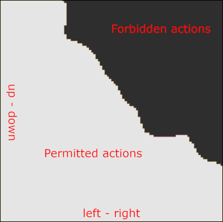
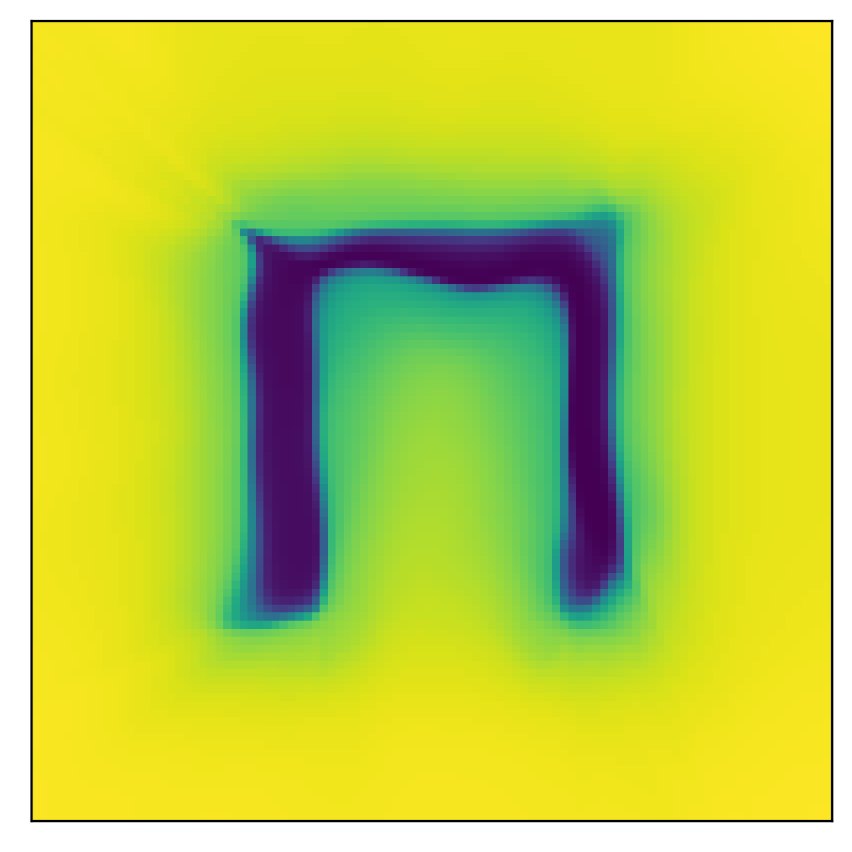
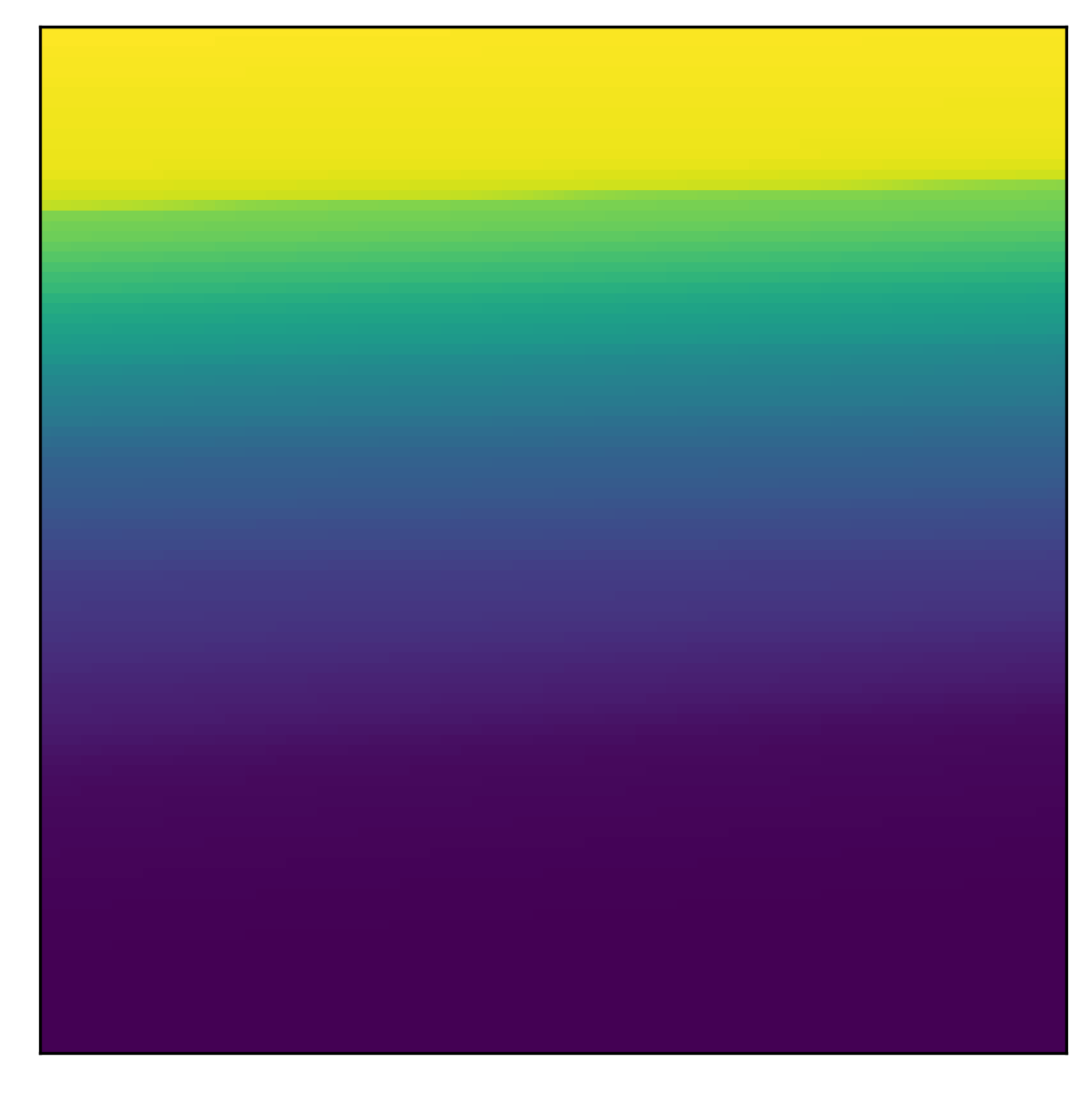
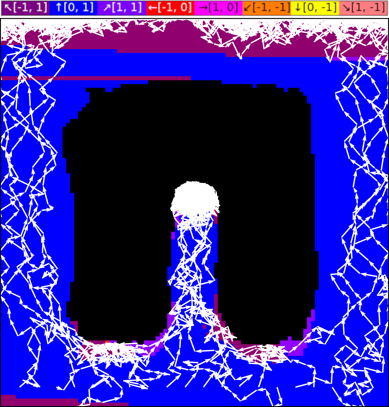
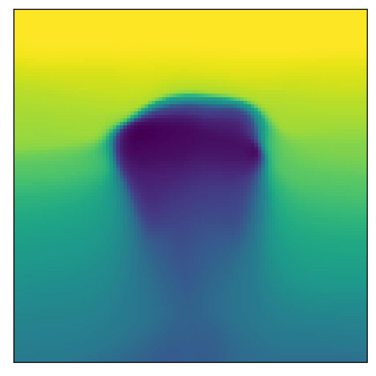
\[\max_{\mathbf{a}^\prime \in \mathcal{A}} Q_i(\mathbf{s}, \mathbf{a}^\prime) - Q_i(\mathbf{s}, \mathbf{a}) \leq \varepsilon_i, \\ \forall \mathbf{a} \sim \pi_\succ, \\ \forall \mathbf{s} \in \mathcal{S}, \\ \forall i \in \{1, \dots, n - 1\}. \tag{9}\]In this form of the lexicographic constraint, action selection, in every state, is constrained to actions whose Q-values are as good as that of the optimal action, minus the threshold \(\varepsilon_i\), for all \(i-1\) higher priority tasks. This makes for a binary mask over the action space, where some subset of actions \(\mathcal{A}_{\succ i}\) is allowed when optimizing task \(r_i\), since it satisfies the above constraint, while the remaining actions are forbidden. In our paper, we refer to this subset as the indifference-space of task \(i\), since with respect to the constraint, the task is indifferent as to which of the near-optimal actions in \(\mathcal{A}_{\succ i}\) is executed. As a concrete example, consider the following images. We have an obstacle-avoidance and goal navigation environment (first image), with a point-mass agent whose 2D action-space corresponds to increments in the \(xy\)-plane. We now train the agent on the first task, i.e. the highest priority task, which here corresponds to avoiding the obstacle. The learned Q-function is shown in the center image. Now, based on the learned Q-function, we can visualize the lexicographic constraint and the indifference space (last image), with the agent placed at the position indicated by the red dot. As can be seen, lexicographic constraint forbids all those actions that would lead to a collision. The remaining, permitted actions can be used for optimizing lower-priority tasks, like navigating to the top goal area.


By relying on the local form of the lexicographic constraint in (9) and the resulting indifference space, we eliminated the need for computing the intractable set \(\Pi_i\) for policy search. This is because instead of computing \(\Pi_i\), the action indifference \(\mathcal{A}_{\succ i}\) gives rise to a new MDP \(M_{\succ i}\), which uses the scalar reward \(r_i\) and whose action space no longer corresponds to \(\mathcal{A}\), but to the indifference space \(\mathcal{A}_{\succ i}\). In this new MDP \(\mathcal{M}_{\succ i}\) we can perform unconstrained policy search to optimize task \(r_i\), since the lexicographic constraint is moved into the action space and thereby always satisfied by construction. This is the short version, the (very cool and intuitive) mathematical derivation and justification of this approach can be found in Section A of the supplementary material of our paper.
Based on this insight, we propose our learning algorithm, Prioritized Soft Q-Decomposition (PSQD), for continuous action-space lexicographic MORL tasks. PSQD combines Q-Decomposition with Soft Q-Learning by first pre-training on all subtasks \(r_1, \dots, r_n\) of the lexicographic MORL problem. This way, we obtain \(n\) soft Q-functions \(Q_1^*, \dots, Q_n^*\) which we can then use to zero-shot the Q-function \(Q_\succ\) of the overall, lexicographic MORL problem. The agent using the zero-shot Q-function \(Q_\succ\) respects the lexicographic constraints, however, it does not behave optimally w.r.t the overall, lexicographic MDP \(\mathcal{M}_\succ\), since the constituent Q-functions \(Q_1^*, \dots, Q_n^*\) were pre-trained separately and suffer from the aforementioned illusion of control. The effect of this can be observed in the following, intermediate result:
Here, the first image again shows the obstacle avoidance Q-function \(Q_0^*\). The second image corresponds the the top goal reaching Q-function \(Q_1^*\). In the last image, we visualize the policy (colored background) and rollouts from the zeroshot agent, obtained as \(Q_{1\succ2} = Q_1^* + Q_2^*\) via Q-Decomposition. As can be seen, the zeroshot agent respects the lexicographic constraint and avoids colliding with the obstacle, but greedily navigates to the top and therefore gets stuck inside the obstacle.
Notice that this result is expected and positive. Due to the lexicographic constraint, we know that the agent can not collide with the obstacle. In our paper, we show that PSQD assigns zero likelihood to actions that violate the lexicographic constraint. This is in stark contrast to standard MORL algorithms that rely on scalarization, meaning that the learned agent’s behavior is largely dictated by reward scale, with zero guarantees on resulting behavior.
However, we are of course interested in obtaining the optimal solution to the overall, lexicographic MORL problem. That’s why PSQD uses the zeroshot composition merely as a starting point and subsequently continues improving performance by finetuning the constituent Q-functions, thereby learning the optimal solution to the overall, lexicographic MORL problem. Concretely, we finetune the constituent Q-functions by iteratively performing soft Q-Learnign in the transformed MDP \(\mathcal{M}_{\succ i}\). Since the highest priority task is not affected by the lexicographic constraint (there are no higher-priority tasks that constrain it), in the first iteration, PSQD finetunes the task with the second highest priority by performing SQL in \(\mathcal{M}_{\succ i}\). This means updating the \(Q_2^*\) to \(Q_{\succ 2}^*\), which is no longer optimal for \(r_2\) but solves \(r_2\) as best as possible while respecting the lexicographic constraint. This involves the following backup operator
\[\mathcal{T}Q(\mathbf{s}, \mathbf{a}) \triangleq r(\mathbf{s}, \mathbf{a}) + \gamma \mathbb{E}_{\mathbf{s}^\prime \sim p} \bigg[ \underbrace{\log \int_{\mathcal{A}_\succ (\mathbf{s}^\prime)} \exp \big( Q(\mathbf{s}^\prime, \mathbf{a}^\prime)\big) d \mathbf{a}^\prime}_{V(\mathbf{s}^\prime)} \bigg], \tag{10}\]where the log-sum-exp expression is not over the entire action space but over the indifference space since we are in the lexicographic MPD \(\mathcal{A}_{\succ i}\). This backup operator is approximated with the following stochastic optimization
\[J_Q(\theta) = \mathbb{E}_{\mathbf{s}_t, \mathbf{a}_t \sim \mathcal{D}} \Bigg[ \frac{1}{2} \Big ( Q^\theta_{n}(\mathbf{s}_t, \mathbf{a}_t) - r_n(\mathbf{s}_t, \mathbf{a}_t) \\ + \gamma \mathbb{E}_{\mathbf{s}_{t+1} \sim p} \big[ V_n^{\bar{\theta}}(\mathbf{s}_{t+1}) \big] \Big)^2 \Bigg ], \tag{11}\]which is the well-known SQL update, with \(V_n^\bar{\theta}\) being the empirical approximation of equation (6) with a target network, parameterized by \(\bar{\theta}\), in \(\mathcal{A}_{\succ i}\). More details about our learning algorithm can of course be found in our paper.
Applying this procedure once to finetune the Q-function of the goal navigation task, we obtain the following result:

Here, the greedy, pre-trained constituent Q-function \(Q_2^*\) in the first image is finetuned as described above, to the optimal constituent Q-function \(Q_{\succ 2}^*\) shown in the second image. Using the finetune Q-function for the second task, we again apply Q-Decomposition to obtain the optimal Q-function for the lexicographic MORL problem as \(Q_\succ^* = Q_1^* + Q_{\succ 2}^*\). The policy and rollouts from this agent are shown in the last image. As can be seen, the agent has learned to avoid the obstacle and to drive out and around it, to reach the top goal area.
The following image shows a visual summary of our learning algorithm, PSQD:
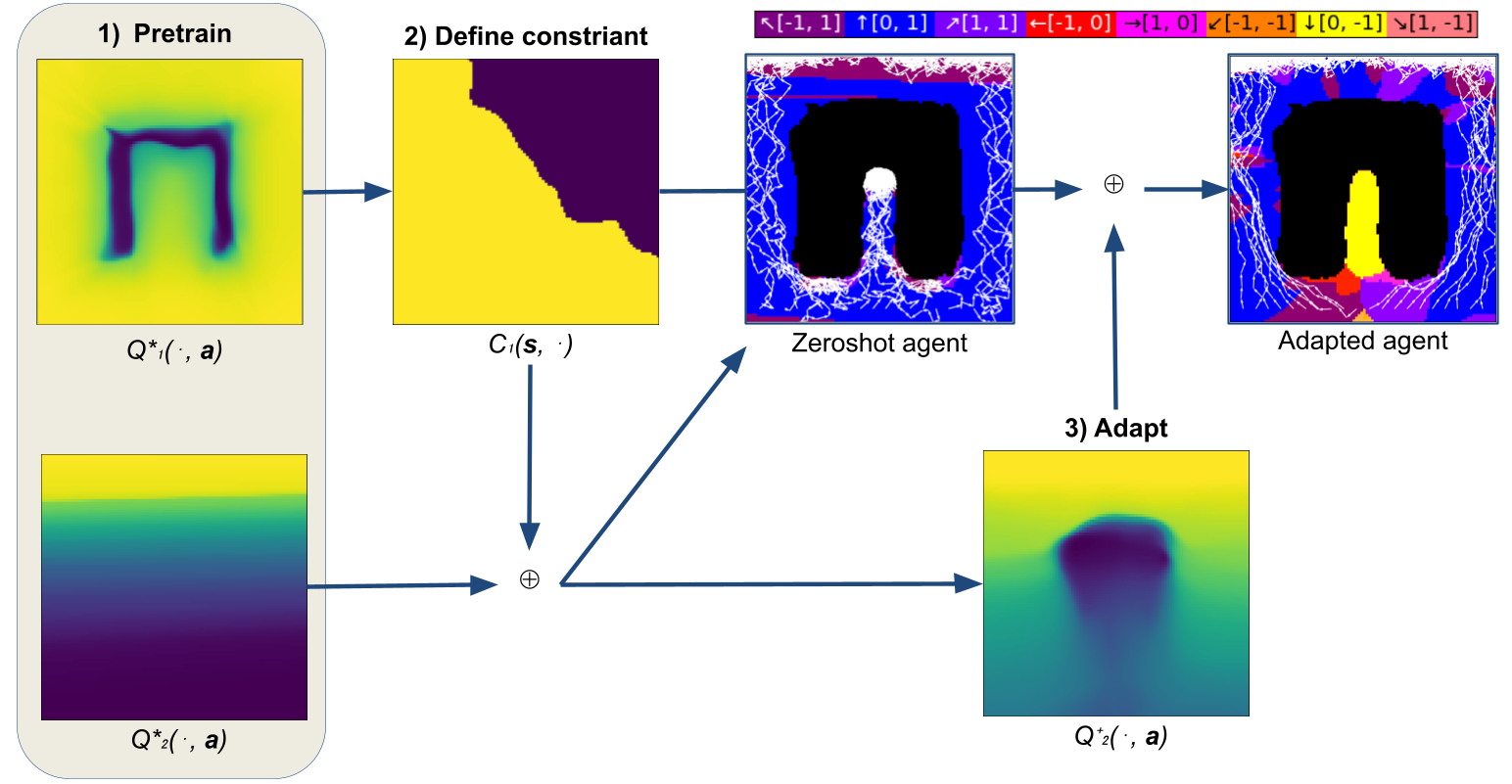
This method trivially extends to more than two tasks. We can add a third subtask \(r_3\), corresponding, for example, to reaching the right-hand side of the environment. With these three subtasks, \(r_1\) for obstacle avoidance, \(r_2\) for reaching the top part of the environment, and \(r_3\) for reaching the right side of the environment, we can make multiple lexicographic MORL problems, by defining different priority orderings. For example, we can keep the highest-priority subtask (obstacle avoidance) fixed but vary the priority of the top- and side-reach subtasks. That is, we can either have the lexicographic MORL problem \(r_{1\succ 2\succ 3}\), where the top-reach subtask \(r_2\) has higher priority than the side-reach subtask \(r_3\), or we can make the lexicographic MORL problem \(r_{1 \succ 3 \succ 2}\), where reaching the side has higher priority than reaching the top.
In either case, we can pre-train on all subtasks separately, and transfer the resulting constituent Q-functions via Q-Decomposition to the lexicographic MORL tasks, where they are subsequently finetuned using PSQD. This results in the following, differing behaviors:
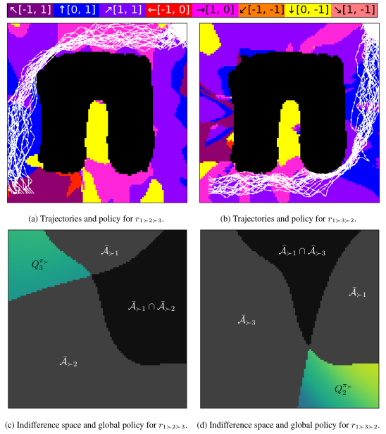
As can be seen, depending on the lexicographic task priority order, the resulting agent either first moves to the top, then to the side in image (a), or first to the side, then to the top, in image (b). The bottom row images visualize the indifference spaces of the constituent Q-functions. Both tasks share the obstacle avoidance component \(\mathcal{\bar{A}}_{\succ 1}\), but have different constraints for the additional task that is varied between the two conditions, \(\mathcal{\bar{A}}_{\succ 2}\) in (c) and \(\mathcal{\bar{A}}_{\succ 3}\) in (d). This aims to illustrate how lexicographic constraints can easily and intuitively be used to induce different, complex behaviors.
Lastly, to demonstrate the efficacy of our method in high-dimensional settings, or, a bit more colloquially, to show that our method scales, we perform a simulated joint-control experiment. Here, the action space is in \(\mathbb{R}^9\) and corresponds to the joint torques of a Franke Emika Panda Robot. The higher-priority task, \(r_1\), corresponds to avoiding a certain subspace of the workspace (red area), while the lower-priority task, \(r_2\), corresponds to reaching a certain end-effector position (green sphere). First, consider a standard MORL algorithm that relies on linear scalarization of the vector-valued reward function. The agent ignores the red area and greedily moves toward the target end-effector position:
This can happen due to poor reward scale or poorly chosen scalarization weights.
Let’s contrast this with our method. We simply define the lexicographic task priority \(o = \langle r_1 \succ r_2\rangle\), set some low threshold, e.g. \(\varepsilon_1 = 1\), and obtain the following (zer-oshot) result:
Here, after separately learning the subtask, even in the zero-shot setting, the agent does not enter the forbidden part of the workspace. To obtain the optimal agent for the lexicographic MORL task, i.e. reaching the target end-effect position while avoiding the forbidden part of the workspace, we perform our finetuning/adaptation step to learn the long-term consequences of the lexicographic constraint. This results in the desired behavior and verifies that our method is also applicable to MDPs with high-dimensional action spaces:
There are some additional, nice properties of our method that I have only mentioned briefly or skipped entirely in this blog post. Firstly, I want to mention how our method benefits sample-efficiency. PSQD transfers knowledge between from simple subtasks to complex, lexicographic MORL problems. Thus, we are not learning the complex, lexicographic MORL problem from scratch, rather, we transfer the pre-trained subtask solutions and perform a simple finetuning step to obtain the optimal solution to the lexicographic MORL tasks. In a nutshell, this implies that we only need to learn once, for example, how to avoid obstacles, we can then re-use this learned behavior every time we want to exploit it as part of a lexicographic MORL problem. Furthermore, each lexicographic task-priority constraints in effect ``shrinks’’ the action/search space of the RL algorithm, which makes it easier to explore the MDP and to discover the optimal solution. Secondly, PSQD respects lexicographic priority constraints even during training and thereby makes for a safe exploration framework. This is again in stark contrast to standard MORL approaches that rely on scalarization and learn each problem from scratch. Lastly, PSQD benefits interpretability of the final agent, since we can inspect the constituent Q-functions and corresponding indifferent spaces to understand the agent’s action selection process.
Summary and conclusion
And that’s it. This blog post presents a short summary of our recent work, Prioritized Soft Q-Decomposition for Lexicographic Reinforcement Learning, which ~is currently under review~ has been accepted at ICLR 2024. The take-away points are as follows:
- Reject scalar reward engineering, and embrace lexicographic task-priority constraints. Lexicographic constraints are much easier to define and have additional benefits, compared to cumbersome, manual tuning of reward scale coefficients.
- Our algorithm, PSQD, solves continuous action-space, lexicographic MORL problems, while explointing the Q-Decomposition method to transfer knowledge from simple subtasks to complex, lexicographic MORL problems.
We are currently working on the successor paper, where we replace soft Q-Learning with a more stable DRL algorithm.
Cheers,
Finn.