Autonomous Navigation with Pepper Robots

Motivation and introduction

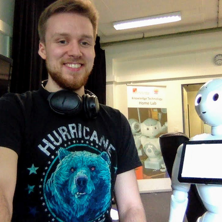
Softbank´s Pepper robot is a popular HRI research platform, however, as already mentioned in my previous post, the onboard LIDAR sensor supplies very sub-optimal data. Unfortunately, the resulting data is essentially useless for running SLAM algorithms because a) it is very sparse with only 15 laser beams and b) due to the awkward angle of those beams, their range is roughly 5 meters. I tried running ros-gmapping with Pepper’s onboard LIDAR sensor and the results were, as expected, not satisfactory. At the KT research group, we wanted to implement autonomous navigation with Pepper robots, which clearly requires good mapping and localization capabilities. Thus, we explored two alternatives to Pepper’s poor onboard LIDAR sensor: We experimented with some visual-slam algorithms, including ORB_SLAM2, but were not satisfied with the results, most likely due to the shaky, blurry, and low-resolution stream of Pepper´s cameras and the relatively featureless environment that is our office building. Thus, exploring another option, we build an external, dedicated sensor system for mapping and localization and rigidly attached it to one of our Pepper robots. This approach turned out to yield good mapping, localization and navigation results and can be reproduced with relatively little monetary cost. This post aims to give guidance to anyone who wants to implement a similar solution for their Pepper robot(s) and explains our method at an intermediately-detailed level.

The high-level approach

The idea of building an external mapping/localization device is motivated by the ROS hector_slam package, made by the folks at TU Darmstadt. This demo video (from 2011), illustrates the capabilities of their algorithm very well:

Given these amazing results on a handheld device, the overall approach is clear: We can simply build a similar hardware system as is used in the video, “duct-tape” it onto our Pepper robot and establish communication between the mapping device and Pepper, such that we can map the environment, then run a localization and navigation algorithm that communicates with the robot to autonomously navigate based on the previously obtained map. Certainly a lot of work but doable. In the following sections, I detail the steps of this approach and attempt to highlight the pitfalls that cost me considerable time along the way.

Hardware components

First of all, if you want to replicate the approach I describe here, you will need to buy the following hardware components:

• Most importantly, we need a proper laser range finder. We experimented with two different sensors: The high-quality Hokuyo UST-10LX (~1300€) and the much cheaper YDLIDAR G2 (~200€). In our office building navigation scenario, we found no significant differences in results between the two, but note that the YDLIDAR G2 only has a range of ~12 meters, which is insufficient for larger, open spaces.
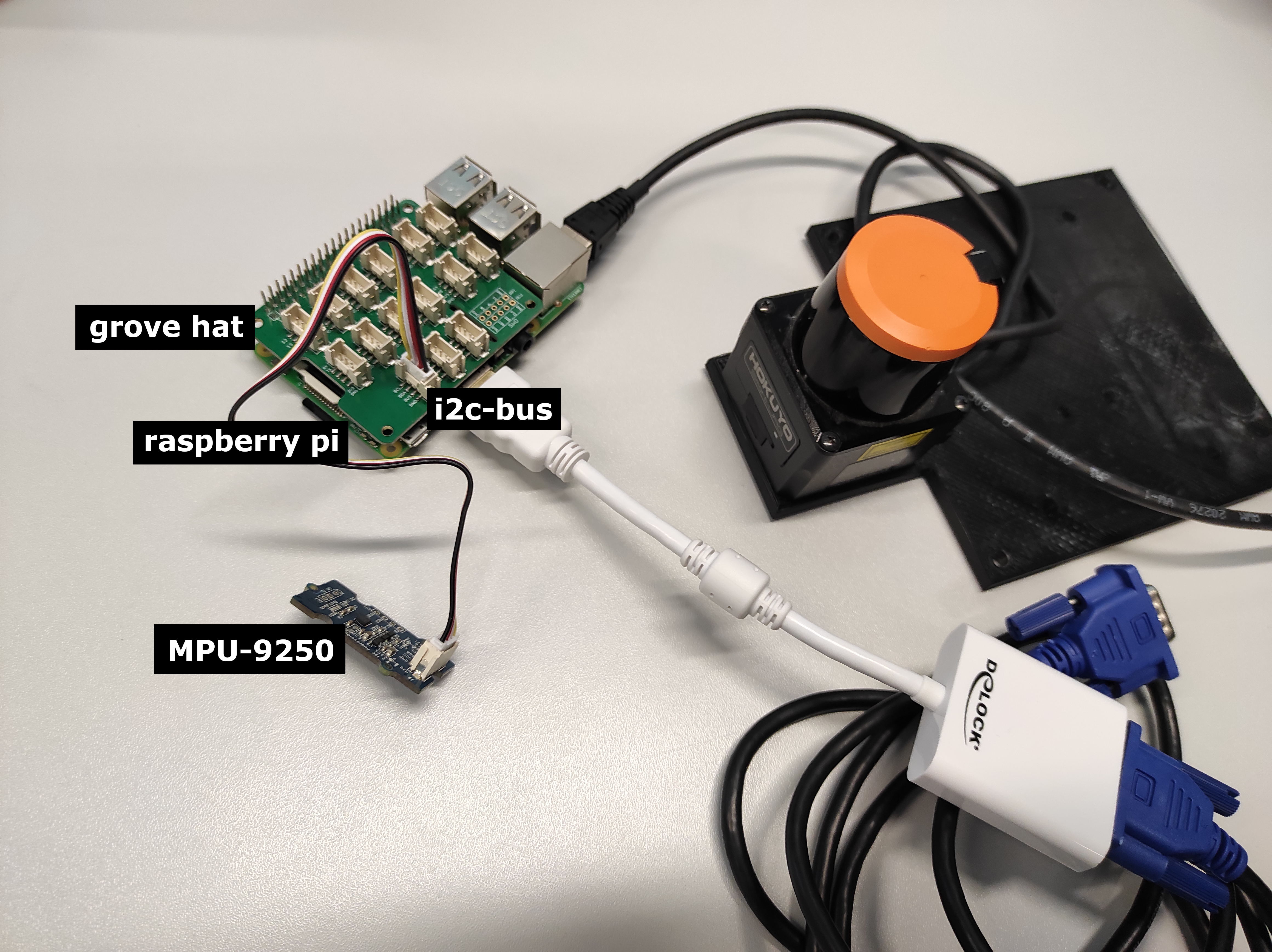
• Additionally, the hector_slam ROS package not strictly requires but benefits from an inertial measurement unit (IMU), which provides acceleration and angular velocity measurements. These are useful when the mapping device is carried around and not rigidly attached to the pepper robot, in which case there can be significant changes in the alleviation and angle of the device, which must of course be considered by the mapping algorithm. Fortunately, IMUs are relatively cheap, we used the MPU-9250 IMU (~15€).
• Furthermore, we require a raspberry pi to stream the sensor data from the IMU and the LIDAR into a ROS network. Our model had 4 GB of RAM and ran a minimal Ubuntu installation. Of course, the more RAM the better, at the time of writing the Raspberry Pi 4 starts at 35€.
• For connecting the MPU-9250 IMU to the raspberry pi we need a special adapter. We used a grove hat adapter (~10€) but this component might be optional, depending on the concrete IMU model you opt for.
• Optionally: You should consider buying a strong battery that powers all of the above components so that you don’t have to attach a power cable to the robot or handheld system during mapping or navigation.
• Lastly, we need some kind of physical framework to actually attach all of these electronics to. We used a set of MakerBeams (starting from 100€), alternative a basic set of LEGO bricks might also work ;)
  

In total, buying all of these hardware components will cost you about 400€. Considering the original cost of one Pepper robot (14.000€+) this is negligible, especially considering that these few components considerably enhance the navigation capabilities of the robot.

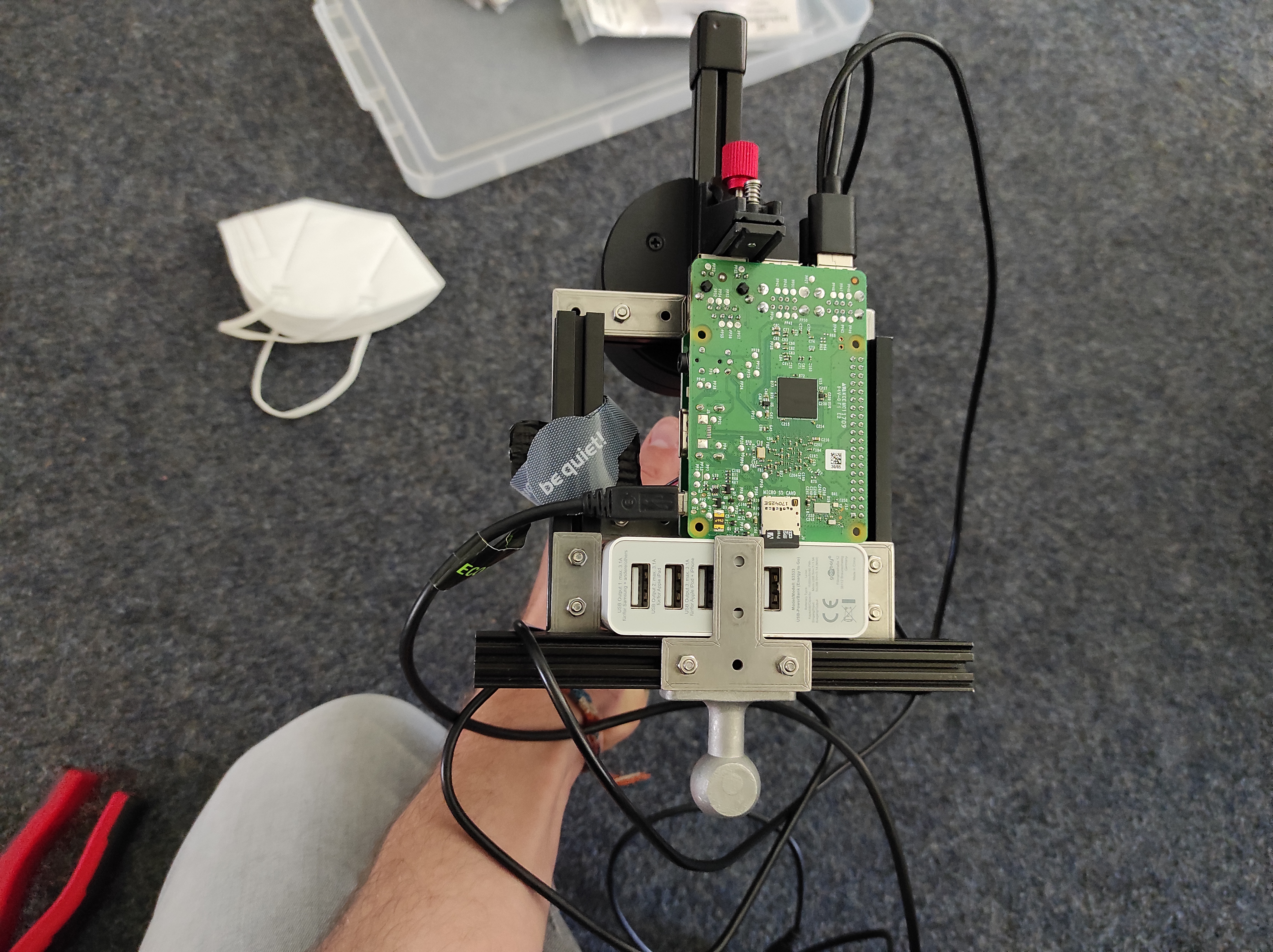
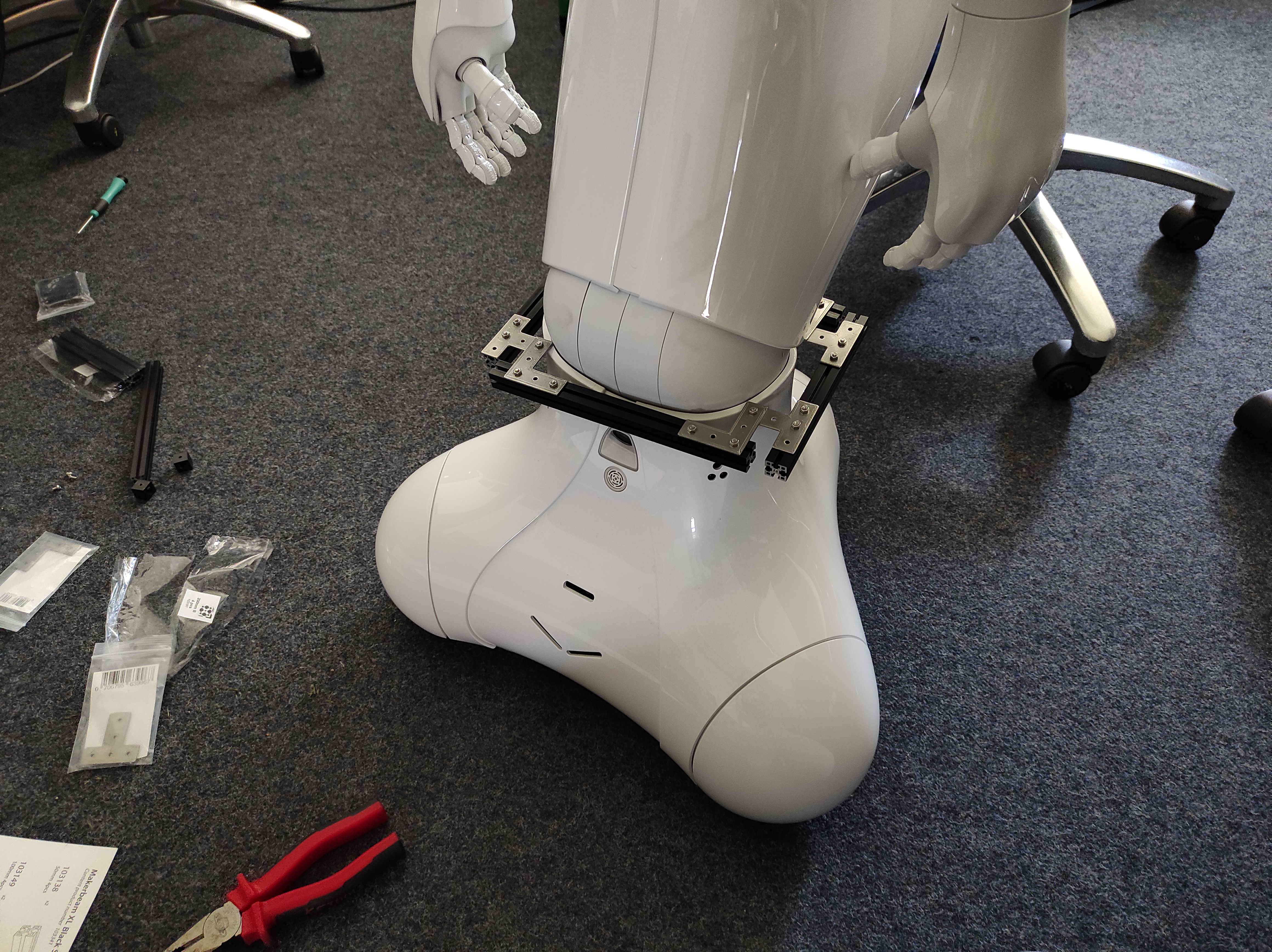
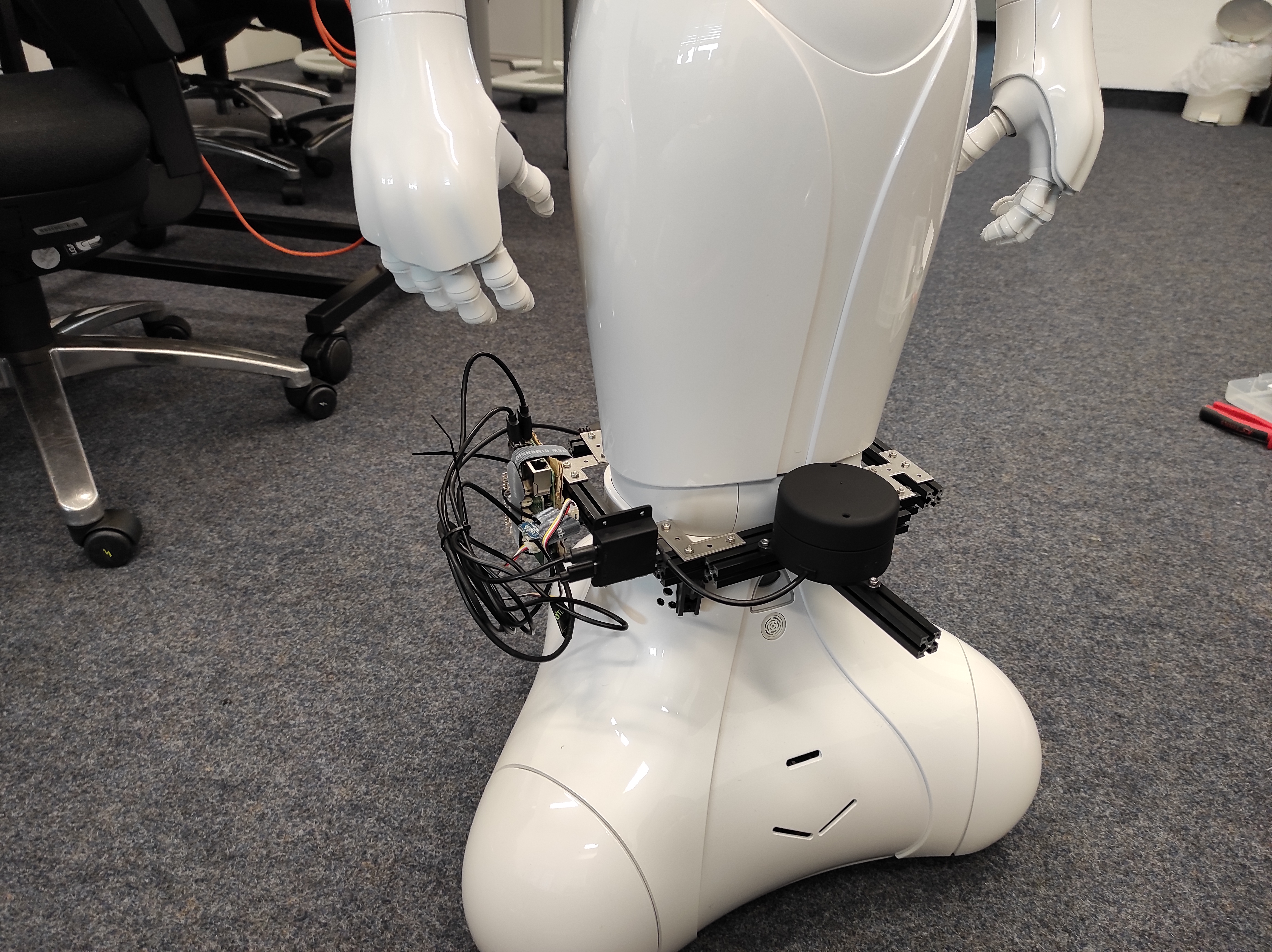
The physical framework

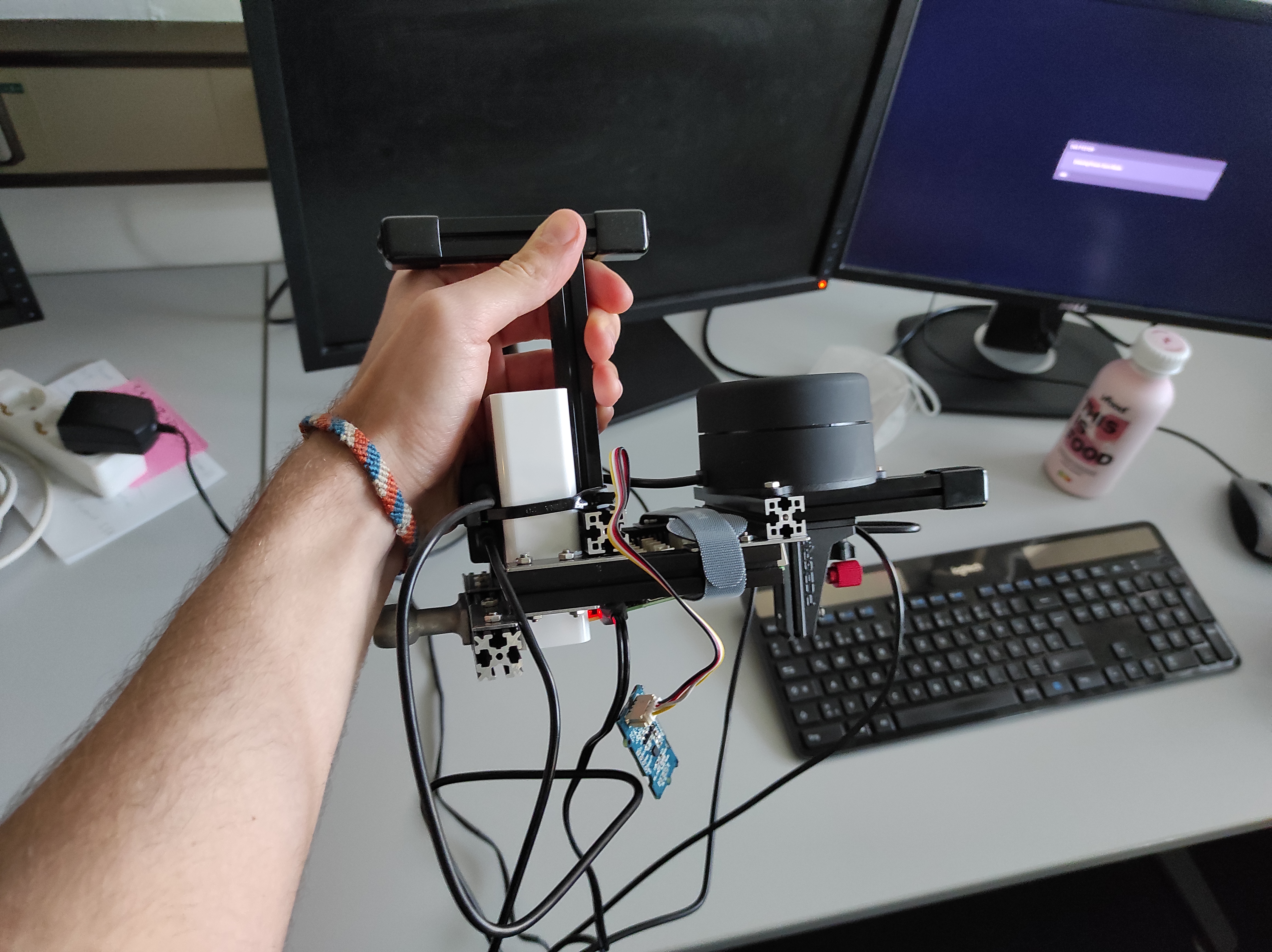
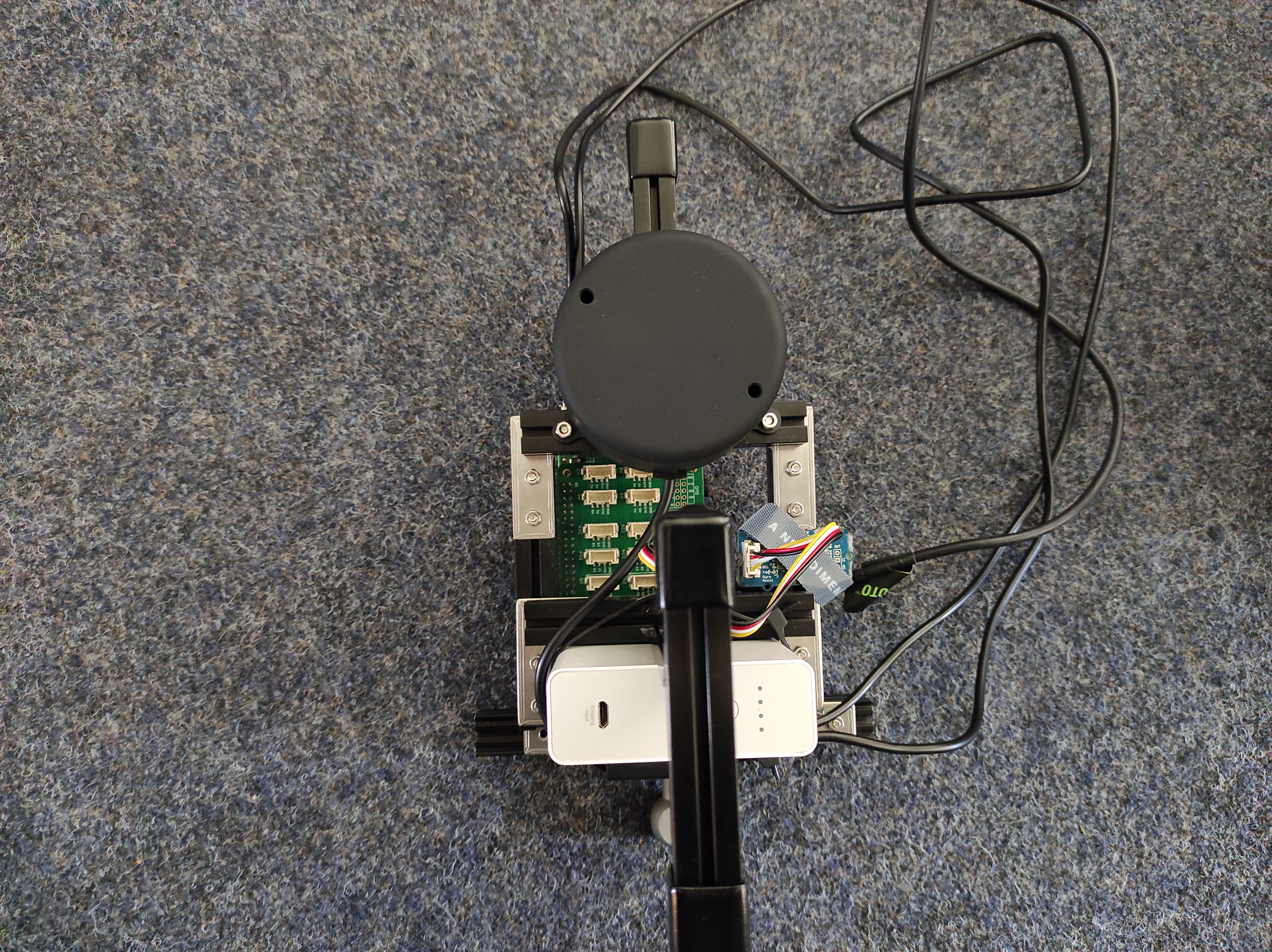
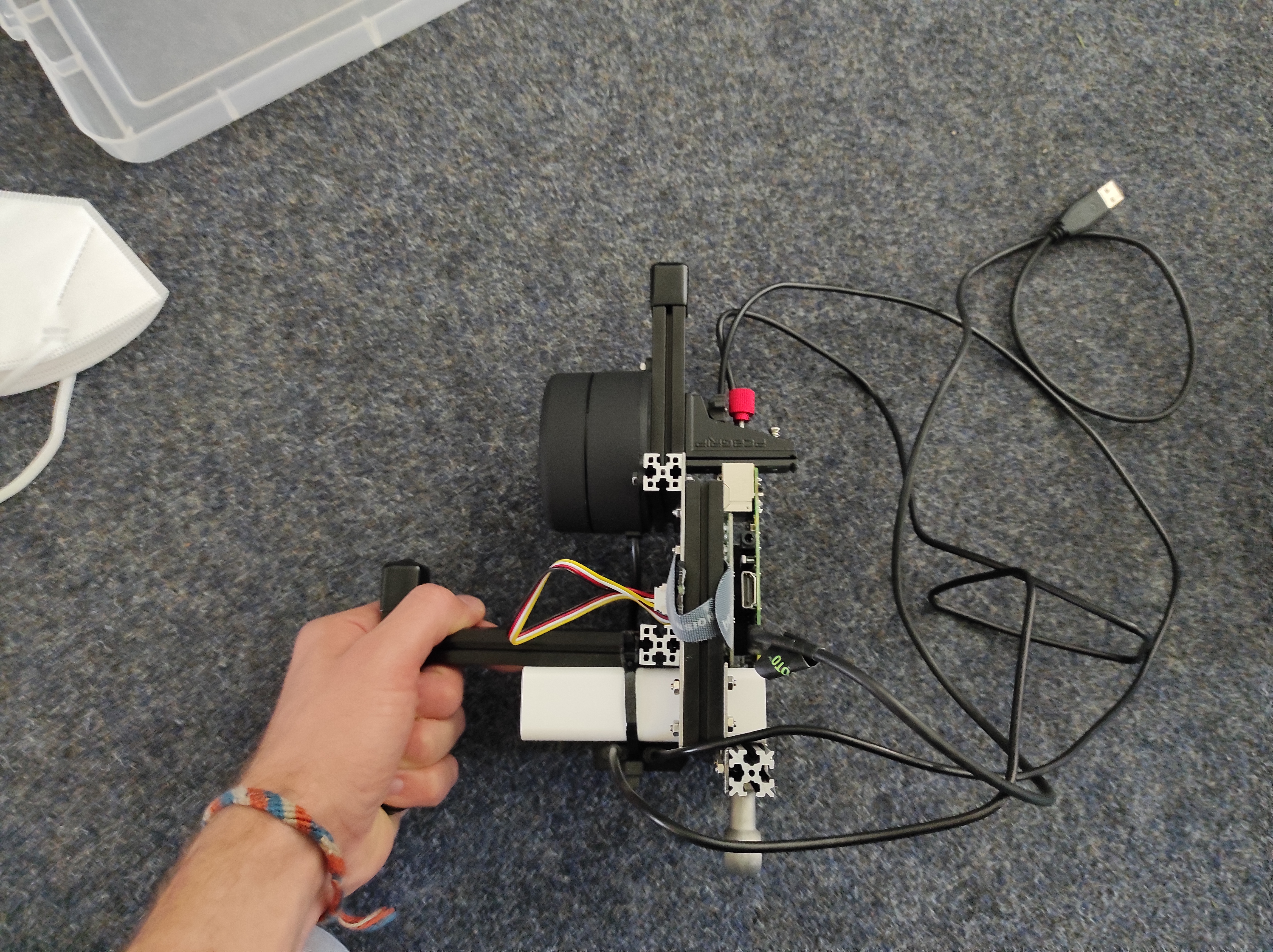
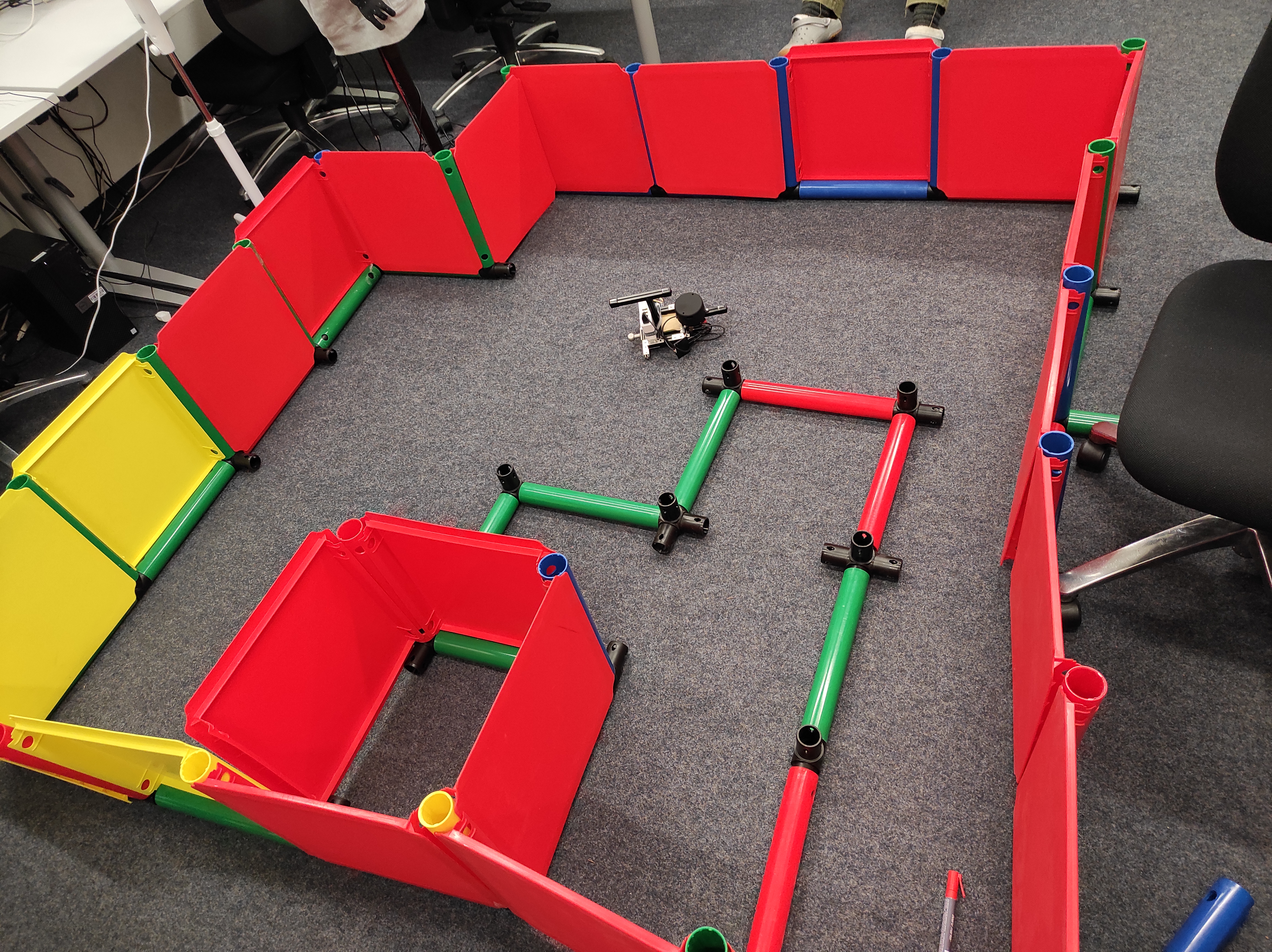
Assuming access to all hardware components, I now describe how to set up the raspberry pi and connect it to the LIDAR and IMU, so that the data from these two sensors will be available for further processing. We ended up building two separate systems. The first one, which we used mainly for debugging, is a direct adaptation of the hand-held device in the demo video above. The second system is a “utility belt” for the Pepper robot, which was eventually used to have Pepper autonomously navigate. Here are images of what these systems looked like:

Physical mapping & navigation device. Either hand-held or attached to Pepper.

Getting LIDAR data

Given a physical construct that holds our sensors, we can start working on the software side of things. First, install your ROS-supporting Linux distro of choice on the raspberry pi. Install a ROS version that supports the drivers and ROS packages required by your IMU and LIDAR sensors. Now, with ROS running on the raspberry, install the drivers and ROS packages required by your LIDAR sensor (also on the raspberry pi). These steps of course depend on the exact sensor you are using. In an earlier post of mine I describe how to set up the Hokuyo UST-10LX LIDAR. For the second LIDAR sensor we were using (the YDLIDAR G2) I will not re-iterate the entire installation process because it is a relatively straightforward and well documented process. However, in short, to get the YDLIDAR G2 to work, you have to

• Connect the YDLIDAR to the raspberry pi as described in the package manual
• install the base SDK
• install the YDLIDAR ROS driver. Don´t forget to replug the YDLIDAR after step 5.

At this point, you should be able to start a roscore on your raspberry pi and launch your LIDAR sensor. You should be able to visualize the data in RVIZ or log the respective ROS topic and confirm that the sensor provides reasonable data. If you are using the YDLIDAR G2, you can call this launchfile to start the sensor. If you are rigidly attaching the mapping device to Pepper, you should consider changing the six values (x y z yaw pitch roll) in line 36 such that they properly reflect the translation and rotation from the parent coordinate frame you are referring to.

Getting IMU data

With you laser scanner (hopefully) providing the desired laser data, we now setup the IMU. This of course also depends on the specific IMU device you are using, but the high-level steps of setting up the MPU-9250 IMU are as follows:

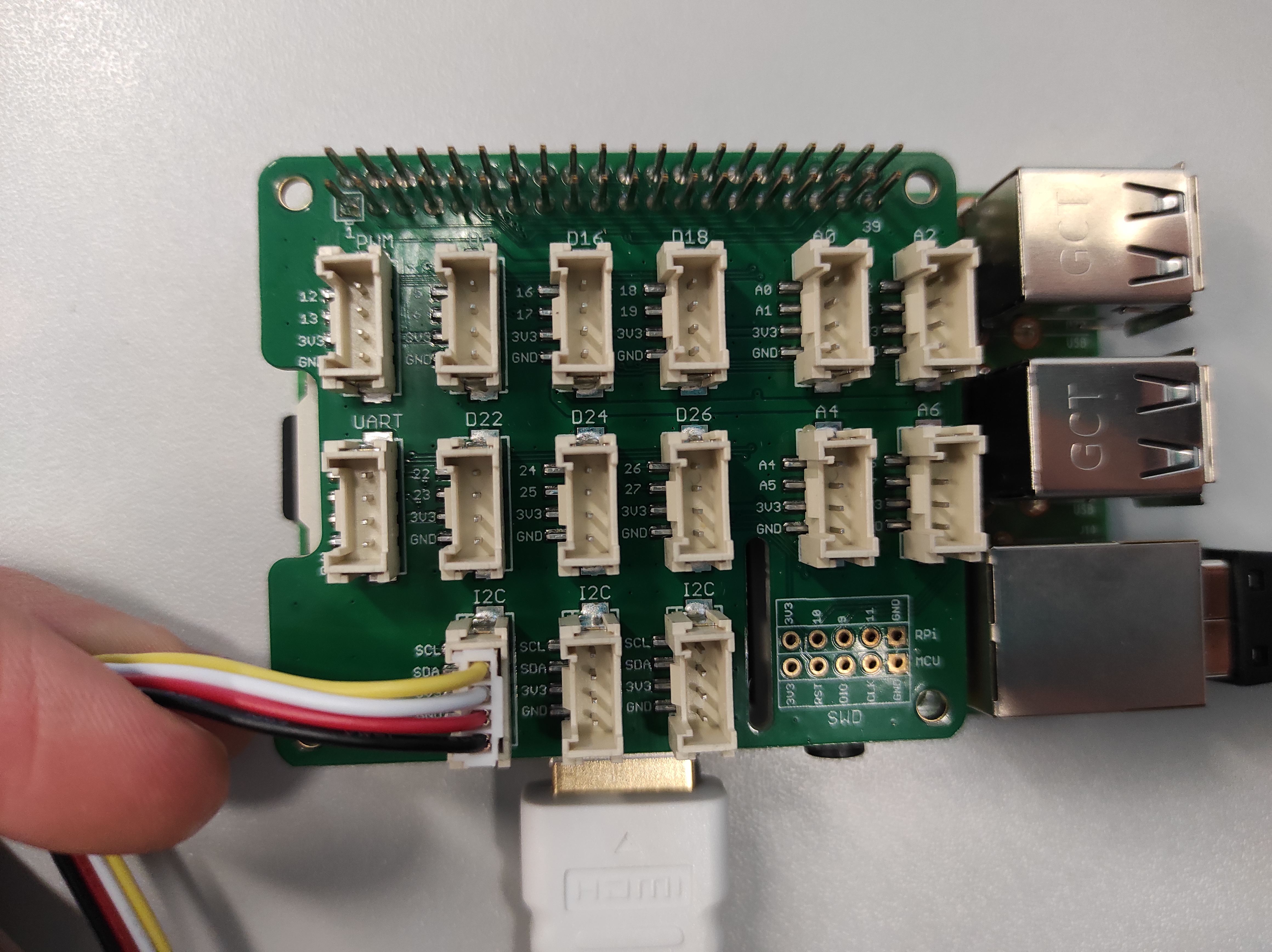
• Connect the IMU to you raspberry pi. If you follow this guide exactly, this involves connecting the grove hat adapter to the GPIO bus of the raspberry pi and installing its driver. Then, connect the MPU-9250 IMU to one of the i2c ports on the grove hat (see picture below).
• Install RTIMULib. Pay attention to the step where you allow non-root users access to the i2c bus, I didn´t read this properly at first, which coused cryptic errors to arise further down the line…
• Install i2c_imu. See this GitHub issue and comment. In the MPU launchfile, for i2c_imu with the MPU-9250 we must set param imu_type to 7. Additionally, I had to set the value for param i2c_bus to 1, which I found out after probing around with the i2cdetect bash tool, which can be installed with sudo apt-get install i2c-tools.

Raspberry pi with grove hat adapter and connected MPU-9250 IMU via I2C bus.

Now, your IMU should be working, and you should be able to access the sensor data with the raspberry pi, similar to this:

Getting TF right

When building a physical system like this, ROS tf errors were the temporary bane of my existence. For people with no background in robotics, it might be somewhat unclear what tf actually does, hence I quickly want to provide some fundamental information: When we wish for robots to assume a certain joint configuration, we must look at the current joint values and then calculate the joint velocities that bring us from the current joint configuration to the desired one. This process is called inverse kinematics. These calculations are not terribly hard to do by hand, but, of course, that´s not what we do, instead, we rely on ROS and its various packages for this. For this to work, the robot must provide a valid “kinematic chain”, which essentially encodes how all the coordinate frames for all the joints are related (i.e. when we move the arm, the attached coordinate frame for the hand will also move). The tf package helps us in managing these different coordinate frames and, most importantly, allows us to easily convert points or vectors between different coordinate frames, given they are linked via a valid kinematic chain.

Why is this relevant? Because we must manually extend Pepper’s kinematic chain such that it can make use of the external IMU and LIDAR sensors and navigate fully autonomously. If we do not set tf up properly, the mapping, localization and navigation algorithms can not interpret the sensor data they are receiving. Just providing the sensor data without the corresponding coordinate frame that is linked to the kinematic chain is not enough because the sensor data points would be missing relative information; they would lack their context. The sensor data lives in a certain coordinate frame, and it must be clear how this frame is related to the rest of the robot in order to do any meaningful computations.

Thus, when mounting the LIDAR or IMU sensor to the robot, make sure you pay attention to the local coordinate frame of the sensor, which might or might not be printed onto the sensor. ROS uses a right-handed coordinate system and the sensor coordinate systems should align with this, i.e. the z-axis is the vertical one, x points to the front and the y-axis points to the left. Thus, when launching your sensors, specify the correct transformation between a sensible parent coordinate frame and the frame of the sensor data. This can be done conveniently via the static transform publisher, for example by including it in the sensor’s launchfile.

Anyway, if you get this wrong, you will quickly notice it, e.g. when the IMU indicates left acceleration when you move it to the right, or because all laser scans are rotated by some degree. In fact, you can see in the IMU video above that the data in RVIZ is no exactly matching what I do with IMU in the real world. This is exactly the issue, the fixed transform that I specified for testing purposes is not in line with the IMU that is just loosely dangling around on my desk, hence the mismatch in orientation.

So, pay close attention when configuring the static transform publisher with the coordinate frames for our IMU and LIDAR. You can read more about the static transform publisher here and, if you want to understand this thoroughly, consider chapter 2 and 3 in Bruno Siciliano’s “Introduction to robotics” book.

Software architecture

Okay, at this point you should have a raspberry pi that is running ROS so that the data from the IMU and LIDAR sensors, which are connected to that raspberry pi, is available via rostopics. In principle, this is enough the replicate the mapping results as shown in the demo video above, via the hector_slam ROS package. I describe the mapping process more in-depth later because for now, I describe our software architecture. Namely, there are two more entities in addition to the sensor-data collecting raspberry pi. Firstly, we have a main ROS server that runs the computationally expensive mapping, localization and navigation algorithms. This way, the raspberry pi only acts as an interface to the sensors and broadcasts the sensor data into a shared local network, but does not have to perform any expensive computations. Secondly, we treat the Pepper robot as another, separate entity that provides sensor data and receives velocity commands. This again has the benefit of not performing expensive computation on the Pepper robot but rather on the main server and secondly, it resolves a very annoying issue: Pepper’s latest ROS packages only support ROS kinetic, which only supports Ubuntu 16. In the following, I describe how to make all of these systems communicate with each other.

Distributed ROS

We have the following three entities:

• A central ROS server (with its own roscore)
• The raspberry pi with attached LIDAR and IMU (with an additional roscore)
• A ROS kinetic docker container that is running Pepper´s ROS stack (running also a dedicated roscore)

To enable these three entities to communicate with each other we require that they all have access to the same local network. This way, the central ROS server can read the topics published by the raspberry pi, process that data (i.e. for mapping or localization and navigation), and output velocity commands that are executed via Pepper’s roscore. In practice, we ran the main roscore and Pepper´s roscore on the same, powerful desktop machine, however, Pepper´s ROS kinetic core was running in an isolated docker container, which resolve the annoying version conflicts (I describe in another blog post how to communicate with a roscore that lives inside a docker container). The key thing to note is that when we have multiple roscores running in the same network, topics provided by the different roscores can be accessed generally, that is a topic from core a can be seen by core b.

Pepper´s docker ROS kinetic core

As mentioned, Pepper´s most recent ROS packages are for ROS kinetic (which released in 2016 and requires Ubuntu 16). The cleanest solution would be to compile all of those packages manually in an up-to-date ROS environment. I tried this and, after wasting a considerable number of hours in this effort, accepted defeat. Thus, I eventually opted for a docker container running ROS kinetic, where Pepper´s ROS packages can be installed straightforwardly. In this docker container, simply install Pepper´s entire ROS stack. Then, you should be able to:

# launch Pepper´s ros driver
roslaunch pepper_bringup pepper_full_py.launch nao_ip:=<YOUR-PEPPER-IP> roscore_ip:=<DOCKER-KINETIC-ROSCORE-IP>  
# the have it assume wake-up pose
rosservice call /pepper_robot/pose/wakeup

of course replacing <YOUR-PEPPER-IP> and <DOCKER-KINETIC-ROSCORE-IP> with the IP address of the Pepper robot and the local ROS kinetics roscore IP address. With a working ROS kinetic environment that allows us to control Pepper through ROS, we must just make sure that we can call services and publish data from our main server and have this take the desired effect in the docker kinetic ROS environment connected to Pepper.

Key configurations for distributed ROS systems

There are two key configurations that are very easy to miss when building a distributed ROS system. I highly consider reading the entire ROS network setup, but nevertheless highlight these two configurations here. Firstly, make sure that the IP address to hostname mapping is properly set up in /etc/hosts. Specifically, for each of our three entities, add the respective other two hostnames and IP addresses to that file. If this is not properly handled, roscore a will only be able to see the rostopics of remote hosts b and c, but the topics will not contain any data (see this thread).

Secondly, the local time for all three entities must be exactly the same. If I recall correctly, the time in the docker container is identical to that on the host, but certainly, the time between the raspberry pi and the desktop machine will not be the same. Here, I mean they must be identical up to a few milliseconds. If they have an offset of e.g. one second, this will cause very weird bugs to occur. For example, I was getting errors from the TF package indicating there was some issue with my kinematic chain, while in fact, the TF messages broadcasted by the raspberry pi were slightly too old (due to the nonidentical time on raspberry and main server), causing the messages to be dropped by the TF instance running on the desktop, even thought the kinematic chain was valid. To fix this, install chrony on the desktop and on the raspberry pi, then synchronize one machine with the clock of the other (both directions should be fine). This process is also documented here.

With these things taken care of, you should now be able to access data from the raspberry pi and from the ROS kinetic core on the main ROS server. You can test this by visualizing the external LIDAR, the IMU and, for example, Pepper´s camera stream in RVIZ on the desktop machine. You should also be able to launch e.g. rqt-steering on the desktop and control Pepper that way. If this works, your distributed ROS system is set up correctly and the navigation algorithm executed on the main server and based on LIDAR data from the raspberry pi will be able to drive Pepper to the desired goal location.

Mapping with hector slam

Given the distributed ROS system described above, the first step towards autonomous navigation is, of course, obtaining a map of the environment. As mentioned initially, here we entirely rely on the hector_slam ROS package. Starting the entire system and creating a map of the environment involves the following steps:

• Start the required sensors (on the raspberry pi they are connected to):
  • Start the IMU (for example by adjusting this launchfile as described above)
  • Start the LIDAR (for example, using this mentioned launchfile)
• Start Pepper’s ROS stack (inside the docker container that communicates with Pepper, as described above)
• On the main server or inside Pepper’s kinetic docker ROS environment, start your tool of choice to control the Pepper robot, i.e. rqt_robot_steering
  Now, we can start the hector_slam ROS package and create a map of the environment.
• Start the hector_slam node (on the more powerful, central ROS server)
  • Start hector_imu_to_tf, this connects the LIDAR data to the angles reported by the IMU
  • Start hector_geotiff, a service for saving the map
  • Optionally, start static_transform_publisher, to ensure that the TF tree is valid and associates all sensor data with the base_link frame
  • Start hector_mapping, the main hector_slam node

Note that there is no difference whether you want to create the map using the hand-held device or with the LIDAR and IMU rigidly mounted to the Pepper robot. This is because the package hector_imu_to_tf links the LIDAR scans to the IMU angles. In practice, this is done by configuring TF in such a way that the laser data frame is the base_stabilized frame, while this frame’s pose is estimated using hector_imu_to_tf package. How hector_slam uses different coordinate frames is further documented here.

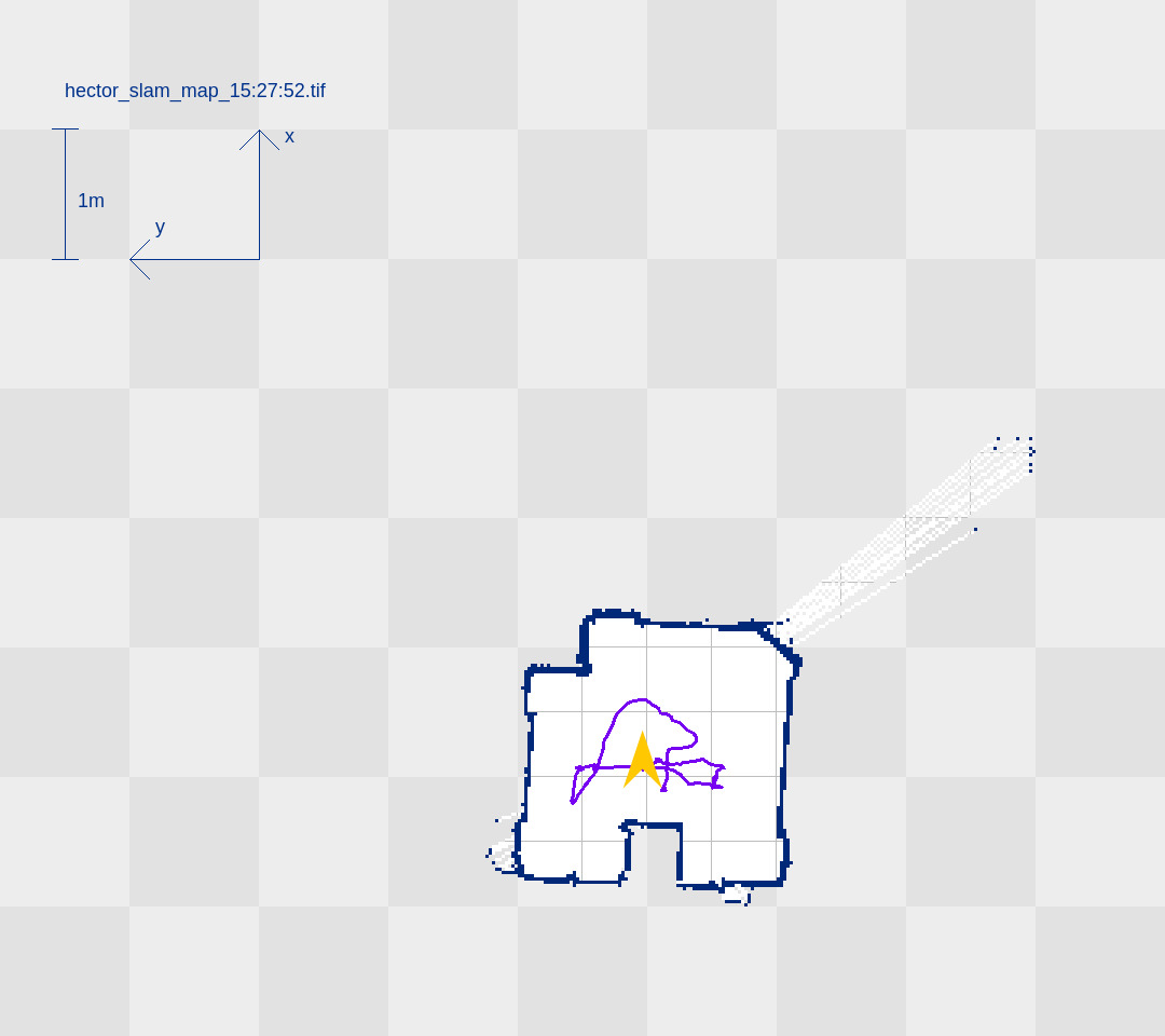
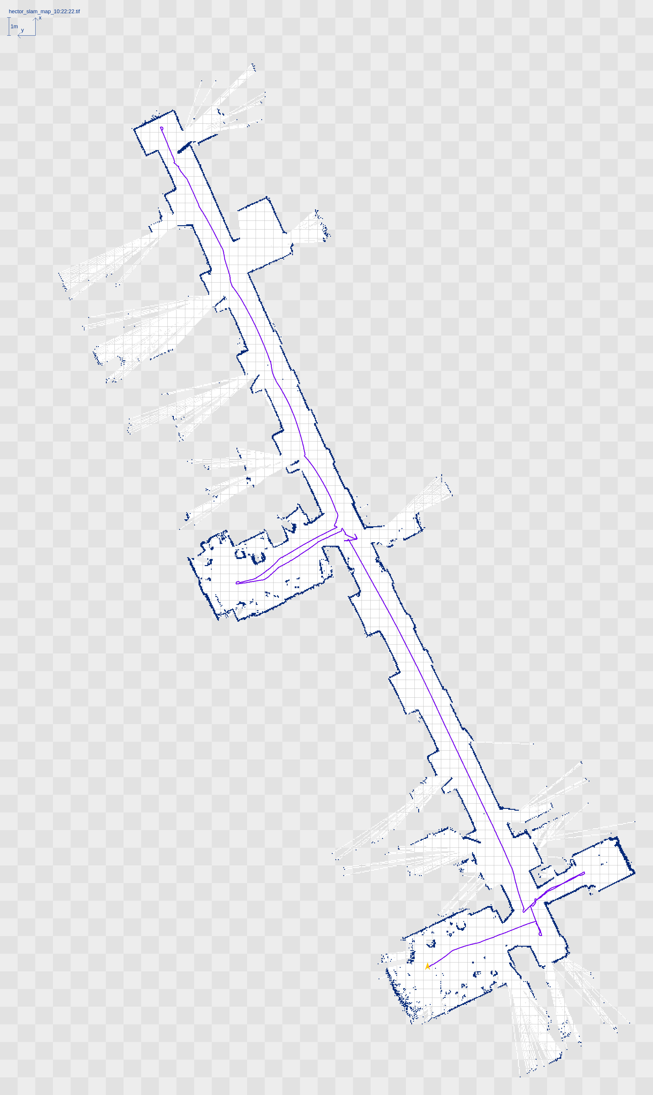
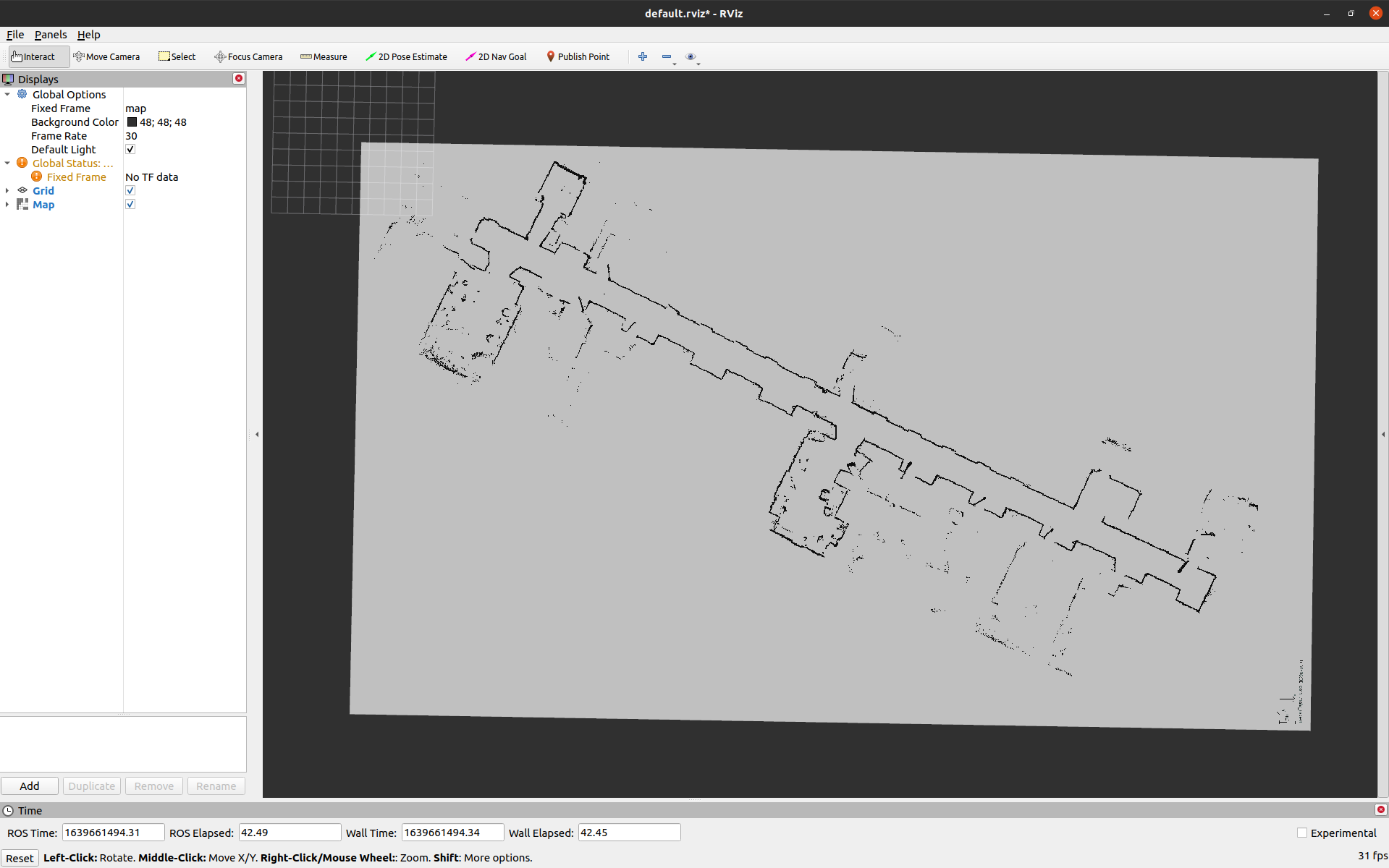
Thus, if everything works, you should be able to obtain good mapping results. Here are exemplary mapping results obtained with the above-described hard- and software-setup. First, we tested and debugged the system in a small, maze-like environment with unique features for easy mapping. Once the system was working well in the test environment, we tested it in the main hallway of our office building and obtained good results.

A small testing environment and mapping results.

Once the entire environment has been mapped, hector_geotiff is used to save the map by executing rostopic pub syscommand std_msgs/String "savegeotiff". This did not work for me immediately and complained with the message “failed with error ‘Device not writable’”. I don’t know the root cause of this, however, I was able to guess a solution relatively quickly. The following command, which re-creates the target folder and takes care of RWX rights fixed the issue for me:
sudo mkdir /opt/ros/melodic/share/hector_geotiff/maps && sudo chmod -R a+rwx /opt/ros/melodic/share/hector_geotiff/maps && sudo chown -R ubuntu:ubuntu /opt/ros/melodic/share/hector_geotiff. Of course, you have to adjust the paths for your ROS installation.

Navigation and Adaptive Monte Carlo Localization

Given a map of our environment, we can now run Adaptive Monte Carlo Localization (AMCL) to estimate the current robot position given a stream of laser scans. You can of course use any other localization algorithm, but the AMCL ROS package generally works very well (if properly parameterized).

Loading hector maps

To start the localization process in a mapped environment, first, we must make the map available on a rostopic. The default topic used for this is accurately called map. The map can be made available by calling the map-server package, which takes as argument the path to a map file, e.g. rosrun map_server map_server path/to/map.yaml. This should make your map available on the map topic, you can check this by either logging the map topic or by visualizing the map topic in RVIZ.

When we load maps that were created with the hector_slam package, we must pay attention to a particular parameter of the map-server package, which took me quite some time to figure out. The maps generated by hector_slam draw obstacles in blue instead of black (as can be seen on the map images above). This causes them to be classified wrongly by the map_server package, because with the default parameters, the blue color is converted to grayscale and happens to fall into an undefined range, meaning the map_server does not identify the blue pixels on the map as actual obstacles. Unfortunately, no warning is raised and the map-server happily broadcasts a map with many invalid (-1) values, which of course makes any localization impossible. This is extra hard to spot, because the resulting map still looks almost perfect when visualized in RVIZ:

The map on the left is valid and can be used for localization and navigation, while the map on the right is invalid and completely useless for localization and navigation. A subtle but devastating difference.

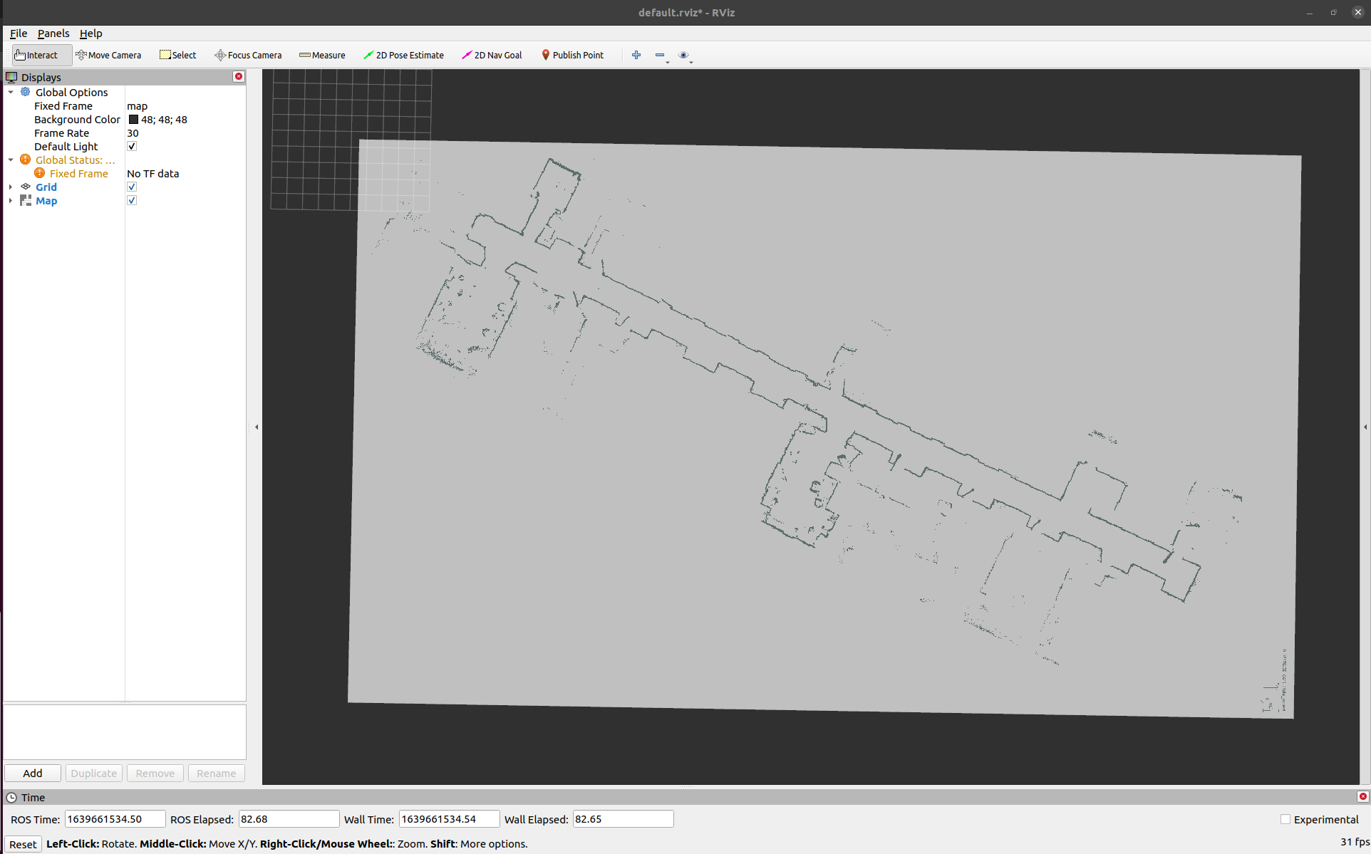
To prevent this from happening, set the parameter occupied_thresh of the map_server package to a lower value, for example, 0.5. The map-server package converts the color values in each cell to a value between 0 and 1, and pixel values greater than occupied_thresh are considered to be an obstacle on the map.

With a correctly loaded map now being available on the map topic, all that’s really left to do now is to start the ACML node. ACML has a lot of parameters, most of which I left at their default values. However, the odometry type should be set to omni via the odom_model_type parameter, since the Pepper robot has an omnidirectional mobile base. Furthermore, the laser_min_range and laser_max_range parameters should match the LIDAR device. For the YDLIDAR G2, I set them to 3 and 16, respectively. Lastly, make sure to pass the correct TF frames to AMCL. This of course is very specific to your TF chain, but most likely you can leave the default values if you didn’t change any TF frame names before.

Store the parameter values in a launchfile and launch AMCL. You can either call the AMCL rosservice global_localization to get an uninformed prior that spreads to pose particles uniformly over the state space or you can use the RVIZ 2D pose estimate button to spread the initial particles normally around the cursor location on the map. Either way, after having initialized the localization algorithm you can (optionally) drive back and forth a bit until the history of laser scans allowed the localization algorithm to converge to the correct position on the map. Alternatively, you can just pass a goal pose and rely on the initial scan history for estimating the initial robot pose.

Based on the given map, current pose and goal pose, navigation is performed by the ROS package move_base, which will calculate a trajectory from the initial pose to the given goal pose. Once this trajectory has been calculated, move_base will output velocity commands on the cmd_vel topic that move the robot along that trajectory to the given target pose. The ROS driver of each specific robot must implement the functionality that interprets and executes the given velocity command with the available robot actuators, like Pepper’s omnidirectional wheels. In our case, Pepper’s ROS kinetic stack implements a velocity controller somewhere, I guess.

And that is it. With a setup like this, we can exploit the powerful ROS navigation stack to autonomously navigate with (slightly modified) Pepper robots. My colleague Dr Phillip Allgeuer continued to work on this project when I had to leave the Knowledge Technology group to start my PhD. Phillip made considerable improvements to our codebase, finalized the project and produced two videos which I slightly edited and combined into the following:

Although I don’t know the following for certain, I hypothesize that the pauses of the robot in the second clip are based on Pepper’s onboard safety features. If enabled, these will override any control if it is considered unsafe, by some criterion. I observed numerous times that Pepper would suddenly stop moving when it is in close proximity to an obstacle, or when it moves at somewhat fast velocities, for example to maintain a safe balance.

Summary

To summarize, we wanted that our Pepper robots could autonomously navigate our office premises. We found that the onboard laser ranger finders did not allow for satisfactory mapping and localization performance. Thus, we extended the Pepper robot with better LIDAR and IMU sensors, which allows us to run the powerful hector_slam package for mapping, and amcl plus move_base for localiation and motion planning/navigation. This required a somewhat sophisticated, distributed hardware, software and network architecture that is described in this blog post for anyone to reproduce.

Cheers,
Finn.