Fun with Graph Neural Networks

Motivation and introduction

Recently, I became interested in Graph Neural Networks (GNNs) because they are a trending topic in the Machine Learning / Deep Learning community. Thus, in this blog post, I briefly introduce and motivate GNNs based on my novice-level understanding of them. Then, I share some results where I analyze and compare GNNs with classical Multilayer Perceptrons (MLPs) on a simple graph classification task.

Graph Neural Networks: What, why, and how?

So what are GNNs, why do we need them and how do they fundamentally work? GNNs are, broadly and informally speaking, Neural Networks (NNs) that can process and exploit non-Euclidean data structures, like graphs.
Classical NNs can not capture and exploit the complex structure of non-Euclidean data because they assume fixed-dimensional, grid-like (aka Euclidean) data. MLPs, for example, assume that their input features come from arbitrary-but-fixed-dimensional, continuous, real-valued (aka Euclidean) vector spaces. Euclidean vector spaces generalize Euclidean geometry (parallel lines never intersect, laws of trigonometry apply) from 2D or 3D to higher-dimensional spaces. Convolutional Neural Networks (CNNs) exploit the Euclidean nature of their input data even more explicitly since they learn local filters that are applied over the entire input space in a sliding-window manner, thereby assuming Euclidean structure. To intuitively see that classical CNNs can not work on non-Euclidean data, consider the following picture:

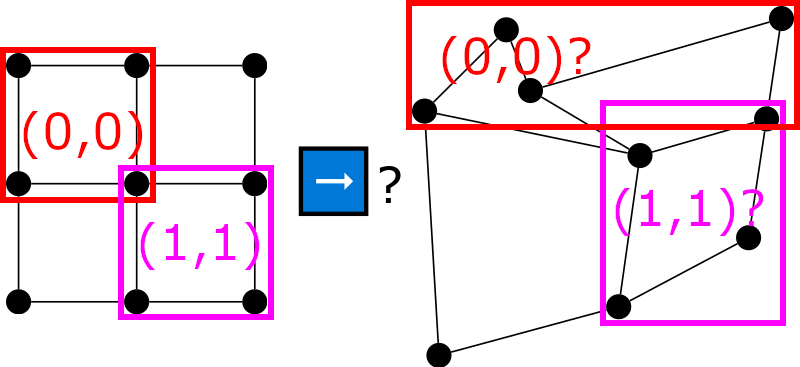
It is clear how to apply 2x2 filters at coordinates (0, 0) and (1, 1) for Euclidean (e.g. image, left) data, but unclear how to do the same for non-Euclidean (e.g. graph, right) data. And this is, essentially, the motivation behind GNNs. Many interesting problems feature non-euclidean data (e.g. graph/node classification, graph/node regression, social network analysis, molecular chemistry, anomaly detection) and we would like to have Neural Networks that can exploit and reason about data from such domains.

With the motivation for GNNs out of the way, let’s see how GNNs work. Note that there are multiple ways of implementing GNNs and that I will only summarize Kipf and Willing’s method in the following, which introduces the Graph Convolution Network (GCN), a particular type of GNN. As the name implies, with the GCN, Kipf and Willing essentially generalize CNNs non-Euclidean data, addressing the issue demonstrated in the image above. At a very high level and as we shall see, this is done by replacing the fixed neighborhood indexing of convolutional filters with a dynamic summation over the neighborhood of vertices in a graph. The GCN operates on a graph \(\mathcal{G = (V, E)}\), where \(\mathcal{V}\) are the graph’s vertices and \(\mathcal{E}\) are the graph’s edges. Each vertex \(\mathcal{V}_i\) in the graph might be described by some \(n\)-dimensional feature vector. Furthermore, \(A\) refers to the adjacency matrix of graph \(\mathcal{G}\), which is a different way of describing the edges in a graph. Let’s skip the theoretical derivation of the GCN (see the paper for details) and jump right to the model definition. Kipf and Willing provide the layer-wise definition of the GCN (in matrix notation) as follows:

\[H^{(l+1)} = \sigma \Big( \underbrace{D^{-\frac{1}{2}} \hat{A} D^{-\frac{1}{2}}}_{\text{normalized } \hat{A}} H^{(l)} W^{(l)} \Big), \tag{1}\]

where \(\sigma\) is a non-linear, differential activation function (e.g. ReLU, GeLU, TanH), \(D_{ii} = \sum_j \hat{A}_{ij}\) (multiplying by \(D\) essentially normalizes \(\hat{A}\)), \(\hat{A} = A + I\) (adding the identity matrix \(I\) to \(A\) is a trick that adds self connections to each vertex in the graph which is beneficial for representation learning), \(H^{(l)}\) is the hidden activation of the previous layer \(l\), and \(W^{(l)}\) is the learnable weight matrix of layer \(l\). ` For input layer \(H^{(l=0)}\) of the GCN we simply have \(H^{(l=0)} = X\), aka the \(n \times d\) -dimensional feature matrix of the Graph \(\mathcal{G}\), where \(d\) corresponds to the number of vertices in the graph and \(n\) to the aforementioned features of vertices. While the above formula specifies the GCN entirely, I find it hard to understand how the GCN works just based on this. So far, this looks almost like the layer of a plain MLP, with the addition of the \(D^{-\frac{1}{2}} \hat{A} D^{-\frac{1}{2}}\) (essentially the normalized adjacency matrix with self-connections), inside of the activation function. How does the GCN deal with the dynamic, non-Euclidean structure of the data? This becomes clear by considering Equation (1) in vector notation (Equation 12 in the paper):

\(h_i^{(l)} = \sigma \Big( \sum_{j \in \mathcal{N}_i \cup \{ i \} } \frac{1}{c_{ij}} \mathbf{W}^{(l)} h_j^{(l-1)} \Big). \tag{2}\)
Here, we can see clearly that the hidden representation of node \(i\) in layer \((l)\) of the GCN is the elementwise non-linear activation of a summation over the neighborhood (with self-connection) \(\mathcal{N}_i \cup \{ i \}\) of vertex \(i\) in the graph, where the neighboring vertices \(j\) are based on the hidden representation \(h_j^{(l-1)}\) of that vertex, transformed by the learnable weight matrix \(\mathbf{W}\) of layer \((l)\) and normalized by \(\frac{1}{c_{ij}}\), with \(c_{ij} = \sqrt{|\mathcal{N}_i|\cdot|\mathcal{N}_j|}\). Thus, the GCN addresses the non-Euclidean data structure by replacing fixed indexing typically performed by convolutions with a dynamic summation over vertex neighborhoods.

A toy graph classification dataset

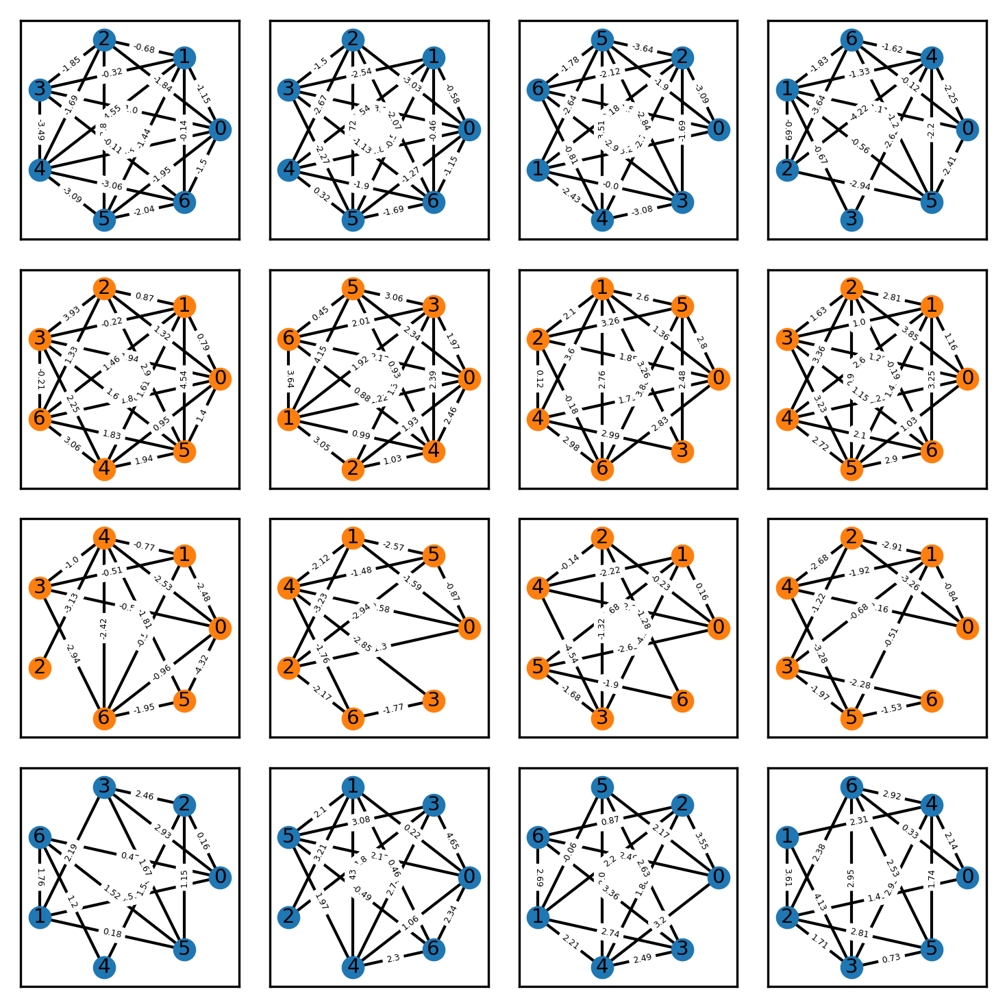
Now that we understand the idea behind GNNs and how GCNs work, let’s put the GCN to the test and see how it compares with a classical MLP on a simple graph classification problem. For this, we need some data. I used the networkx library to create a dataset of random graphs. To make for a binary classification problem, graphs of class 1 have edge probability of 0.4, while graphs of class 2 have edge probability 0.6, thus the two graph classes have differing degrees. Similarly, I varied the edge weights between the two classes, such that graphs of class 1 randomly draw their edge weight from a standard Gaussian with mean -2, while graphs of class 2 draw their edge weight from a standard Gaussian with mean 2. These (scalar )edge features can trivially be encoded by the adjacency matrix. This toy dataset essentially mimics the well-known XOR classification problem, except data points are graphs. Exemplary graphs from this dataset are shown below, where the vertex color indicates the class label.

Let’s now train a vanilla MLP and a GCN on this dataset and see how they compare. I made sure that all graphs in the dataset are of size 7 such that the adjacency matrix is always \(7 \times 7\), which is convenient because otherwise, we would have to perform some preprocessing, e.g. padding, to ensure that the input layer of the networks fits all graphs.

Results

I now briefly describe the MLP and the GCN that were used to generate the following results. As a first step, I created unregularized networks to make sure that I could overfit the dataset. I used the PyTorch Geometric library for the GCN implementation since it provides the GCN layer out of the box. Both the MLP and GCN had two hidden layers of width 64 and had a similar number of learnable parameters, 8962 for the GCN and 7490 for the MLP. I optimized both networks with Adam for 100 epochs, using a batch size of 16. The results for this setting are shown in the following plot:

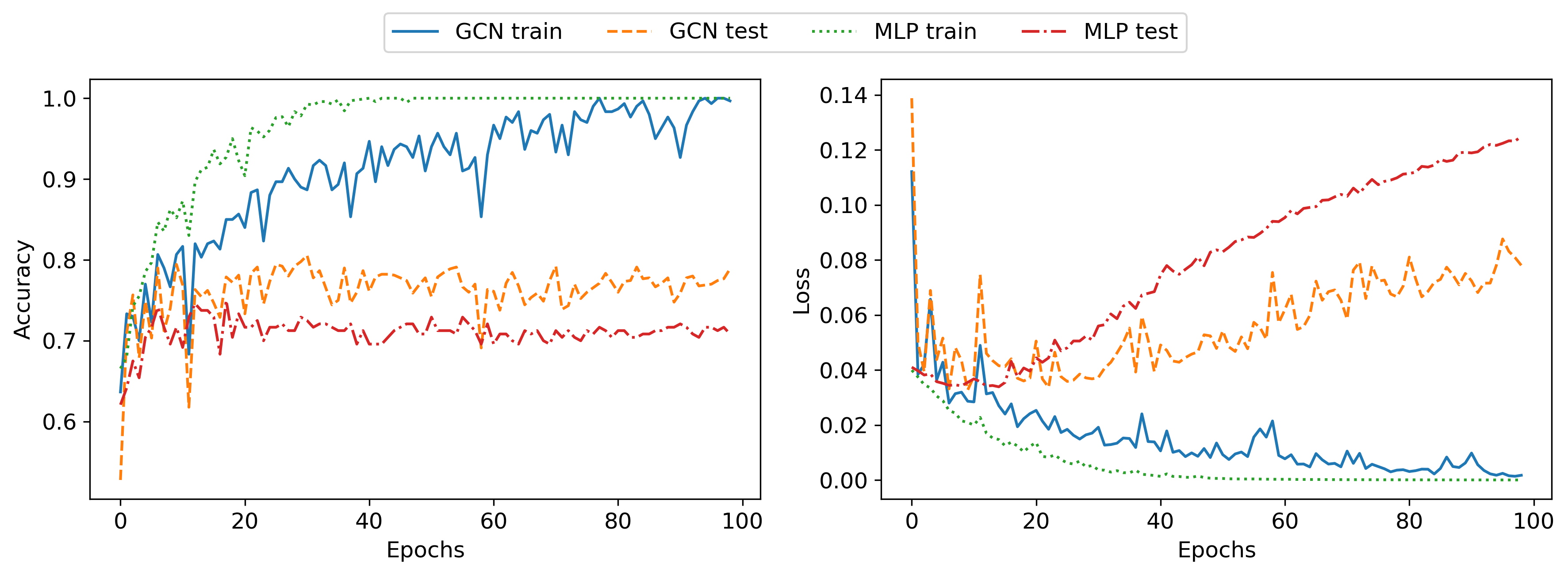
As can be seen, both networks are able to overfit the training set perfectly, achieving 100% classification accuracy. As expected due to the lack of regularization both networks fail to generalize well to the testing set, with the MLP achieving roughly 70% and the GCN 80% classification accuracy. The slightly better generalization as well as the lower testing error of the GCN is probably due to the strong inductive bias of the GCN, compared to the MLP.

Next, I wanted to improve the generalization of these networks. I first chose a few different hyperparameter sets manually but found it very hard to improve accuracy on the test set. I added dropout layers and weight decay for regularization, tried bigger and smaller networks, different batch sizes, and different optimizers, but nothing significantly improved the test set accuracy. The following plot shows results with deeper networks (5 hidden layer of width 32), 50% dropout, and Adam weight decay 1e-4:

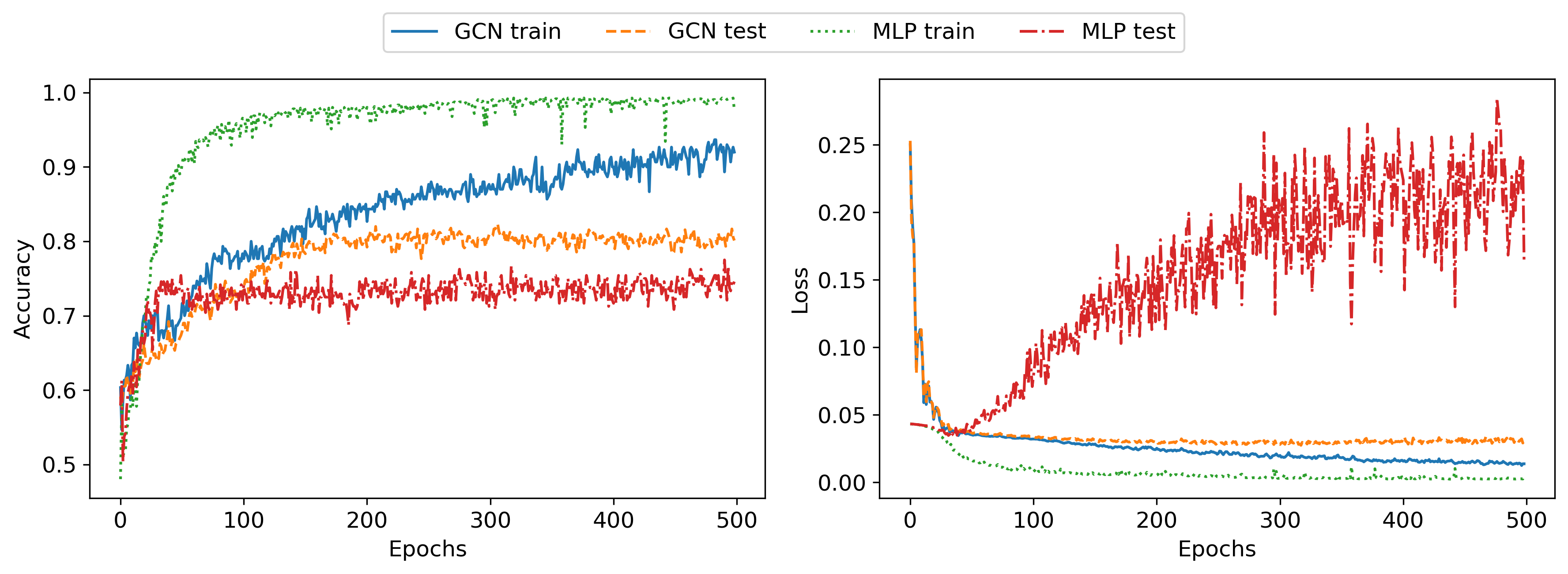
The results show similar patterns as in the unregularized case. Next, I ran a Bayesian hyperparameter optimization for an afternoon, but even that failed to come up with better hyperparameters. This implies that there is some ambiguity in the data that can not be learned, only memorized in the training data. This makes sense since, given the dataset that I created, both edge weight and edge probabilities are sampled randomly and have some overlap, meaning there exists a certain subset of graphs in the dataset that are very hard or impossible to classify correctly, without additional information. It would be interesting to explore the uncertainty of the neural network predictions (for example through monte carlo dropout), but I haven’t done that for this post.

Summary and conclusion

The main takeaway points from this post should be the following: GNNs are neural networks that can exploit non-Euclidean data structures. The GCN generalizes CNNs to non-Euclidean domains by replacing the fixed filter indexing with a dynamic averaging over some proximity neighborhoods. On the graph XOR classification problem, we observed better generalization and less overfitting due to stronger inductive bias by the GCN, compared to an MLP. This last point should be taken with a grain of salt though, since it’s not clear whether it holds generally or just for the specific problem and data used here.

And that’s it, I hope you found this post interesting :)

Cheers,
Finn.